Updated T-MSBL code

I just now updated the T-MSBL/T-SBL code. So, using the updated version, you need NOT to consider the tuning of parameters for a general compressed sensing problem. By a general compressed sensing problem, I mean the columns of the matrix A has unit L2-norm. When your problem does not satisfy this, you can first transform your original problem:
Y = A X + V
to
Y = A W W^{-1} X + V  = A' X' + V
such that A' has unit-norm columns. Once you obtain the result, you can obtain X by X = W X'.


 The calling of T-MSBL is easy:

o   When noise is large (e.g. SNR <=6 dB)

X_est = TMSBL(A, Y, 'noise', 'large')

o   When noise is mild (e.g. 7 dB <= SNR <=22 dB)

X_est = TMSBL(A, Y, 'noise', 'mild')

o   When noise is small (e.g. SNR >22 dB)

X_est = TMSBL(A, Y, 'noise', 'small')

o   When no noise

                                     X_est = TMSBL(A, Y, 'noise', 'no')

But note that the above number 6dB or 22dB is not an exact value. The two values just give you a rough concept of what is the 'small noisy case', what is the 'mild noisy case', and what is the 'strongly noisy case'.
In this sense, this does not mean T-MSBL requires to know the noise level.

When you use T-MSBL in some practical problems when you really have no idea what is the range of noise strength (such as gene feature extraction), simply use the calling corresponding to the 'mild noise case', i.e.

X_est = TMSBL(A, Y, 'noise', 'mild') 

I will update the code in the near future, such that in any case(noisy, noiseless, real variable, complex variable, large-scale data or small-scale data)  you only need to input X_est = TMSBL(A,Y). But I currently am very busy on my on-going papers (four journal papers in three fields), so please forgive me that I cannot do this now.

Minisymposium on New Dimensions in Brain-Machine Interfaces at UCSD

Wednesday, November 9, 2011
1pm-6pm
Fung Auditorium
Powell-Focht Bioengineering Hall
UC San Diego

The minisymposium highlights latest advances and emerging directions in
brain-machine and neuron-silicon interface technology and their
applications to neuroscience and neuroengineering.  Topics include
high-dimensional EEG and ECoG systems, wireless and unobtrusive
brain-machine interfaces, flexible bioelectronics, real-time decoding of
brain and motor activity, and signal processing methods for intelligent
human-system interfaces.


PROGRAM

1:00-1:10pm    Welcome

1:10-1:50pm    Engineering hope with biomimetic systems
              Wentai Liu, UC Santa Cruz

1:50-2:30pm    A low power system-on-chip design for real-time ICA based BCI applications
              Wai-Chi Fang, National Chiao-Tung University, Taiwan

2:30-3:10pm    Developing practical non-contact EEG electrodes
              Yu Mike Chi, Cognionics

3:10-3:50pm    A new platform for BCI: from iBrain to the Stephen Hawking project
              Philip Low, Neurovigil


3:50-4:20pm    Coffee break


4:20-5:00pm    Interdisciplinary approaches to design high performance brain-machine interfaces
              Todd P. Coleman, UC San Diego

5:00-5:40pm    Evolving data collection and signal processing methods for intelligent human-system interfaces
              Scott Makeig, UC San Diego

5:40-6:00pm    Panel discussion


Organized by:

Tzyy-Ping Jung <tpjung@ucsd.edu>
Center for Advanced Neurological Monitoring,
Institute of Engineering in Medicine <http://iem.ucsd.edu>, and
Institute for Neural Computation <http://inc.ucsd.edu>

With support from:

Qualcomm <http://www.qualcomm.com>, and
Brain Corporation <http://www.braincorporation.com>

Compressed Sensing Work by My Friends and Colleagues

Recently some of my friends and colleagues sent me their recent work on compressed sensing/sparse signal recovery. Thanks them for keeping me informed! Here are their nice work: I welcome everybody send me his/her work and I would like to introduce his/her work in my blog :)

Hakan informed me of his work:
Karahanoglu, N.B., and Erdogan, H., “Compressed sensing signal recovery via A* Orthogonal Matching Pursuit,” ICASSP’11, Prag, May 2011.
 The journal version is:
Karahanoglu, N.B., and Erdogan, H., “A* orthogonal matching pursuit: best-first search for compressed sensing signal recovery,” submitted, available as: arxiv 1009.0396,  last update in Sep. 2011.
 Matlab code can be downloaded here. 

The abstract reads:

Compressed sensing aims at reconstruction of sparse signals following acquisition in reduced dimensions, which makes the recovery process under-determined. Due to sparsity, required solution becomes the one with minimum ℓ0 norm, which is untractable to solve for. Commonly used reconstruction techniques include ℓ1 norm minimization and greedy algorithms. This manuscript proposes a novel semi-greedy approach, namely A* Orthogonal Matching Pursuit (A*OMP), which performs A* search for the sparsest solution on a tree whose paths grow similar to the Orthogonal Matching Pursuit (OMP) algorithm. Paths on the tree are evaluated according to an auxiliary cost function, which should compensate for different path lengths. For this purpose, we suggest three different structures. We show that novel dynamic cost functions provide improved results as compared to a conventional choice. Finally, we provide reconstruction results on both synthetically generated data and images showing that A*OMP outperforms well-known CS reconstruction methods, Basis Pursuit (BP), OMP and Subspace Pursuit (SP).

Kiryung informed me of his latest updated work:

Kiryung Lee, Yoram Bresler, Marius Junge, Subspace Methods for Joint Sparse Recovery, arXiv:1004.3071v4

The abstract reads:
We propose robust and efficient algorithms for the joint sparse recovery problem in compressed sensing, which simultaneously recover the supports of jointly sparse signals from their multiple measurement vectors obtained through a common sensing matrix. In a favorable situation, the unknown matrix, which consists of the jointly sparse signals, has linearly independent nonzero rows. In this case, the MUSIC (MUltiple SIgnal Classification) algorithm, originally proposed by Schmidt for the direction of arrival problem in sensor array processing and later proposed and analyzed for joint sparse recovery by Feng and Bresler, provides a guarantee with the minimum number of measurements. We focus instead on the unfavorable but practically significant case of rank-defect or ill-conditioning. This situation arises with limited number of measurement vectors, or with highly correlated signal components. In this case MUSIC fails, and in practice none of the existing methods can consistently approach the fundamental limit. We propose subspace-augmented MUSIC (SA-MUSIC), which improves on MUSIC so that the support is reliably recovered under such unfavorable conditions. Combined with subspace-based greedy algorithms also proposed and analyzed in this paper, SA-MUSIC provides a computationally efficient algorithm with a performance guarantee. The performance guarantees are given in terms of a version of restricted isometry property. In particular, we also present a non-asymptotic perturbation analysis of the signal subspace estimation that has been missing in the previous study of MUSIC.

This is the fourth version. I read its third version, which has about 30 pages. However, the fourth version doubles the page number. So I asked Kiryung what are the main changes compared to the previous version. Kiryung replied:

"We added another subspace greedy algorithm for partial recovery step. This ends up with better empirical performance.  All algorithms presented in this paper have guarantees.  We updated the analysis by using a version of RIP,  which is different from the original uniform RIP and is satisfied by a weaker condition.  "



Justin sent me his journal paper on MMV model using AMP. It's a very cool algorithm. However, the journal paper has not been opened to the public. But I think you can read his conference paper soon:

J. Ziniel and P. Schniter, ``Efficient Message Passing-Based Inference in the Multiple Measurement Vector Problem,'' to appear in Proc. Asilomar Conf. on Signals, Systems, and Computers (Pacific Grove, CA), Nov. 2011.

-------------------------------------
Image: Nepenthes. hamata grown in my patio.

Call for Paper: Special Issue on Dependent Component Analysis

There will be a special issue on Dependent Component Analysis in EURASIP Journal on Advances in Signal Processing.  Dependent component analysis (DCA) is a big extension of ICA, and is one of the main directions of the ICA field in recent years.  I think this issue should be a good window to see current progress on DCA.

The issue includes the following topics (but not limited to):
- Multidimensional component analysis
- (Independent) subspace analysis
- Vector component analysis
- Correlated component analysis
- Topographical component analysis
- Tree-dependent component analysis
- Blind dependent component analysis
- Informed (Bayesian) dependent component analysis
- and their applications

Manuscripts Submission Date:  Feb 1, 2012.
Publication date: Oct.1, 2012.


--------------------------------------------------------
Image: Nepenthes.talangensis, grown in my partio.

How people in science see each other

Today Tobias sent us a picture titled "How people in science see each other". It is very funny.  Enjoying! (click the picture for larger view)

Noise Folding Puts Tough Requirements on Compressed Sensing Algorithms?

Tonight I read two papers on noise folding in the compressed sensing problem. They are:

[1] M.A.Davenport, J.N.Laska, J.R.Treichler, R.G.Baraniuk, The Pros and Cons of Compressive Sensing for Wideband Signal Acquisition: Noise Folding vs. Dynamic Range. Preprint, April, 2011

[2] E.Arias-Castro, Y.C.Eldar, Noise Folding in Compressed Sensing, IEEE Signal Processing Letters, vol.18, no.8, 2011

The noise folding is a silent topic in the hot compressed sensing field. The problem is described as follows:
y = A (x + n) + v                 (1)
Namely, the signal itself contains noise (called 'signal noise' or 'source noise'). v is the measurement noise. The model can be rewritten as
y = Ax + (An+v) = Ax + u.   (2)
Intuitively, the 'noise' has increased, and this will bring "troubles" to algorithms.

The above two papers rigorously analyze how the signal noise n affects the estimation quality, the RIP condition, and so on.

In [1], the authors consider the case when the matrix A is orthonormal and v is not present. They found that the noise folding has a significant impact on the amount of noise present in CS measurements; every time one doubles the subsampling factor g (i.e. the ratio of column number of A to its row number), the SNR loss increases roughly by 3dB, namely,

In [2] the authors considered a general case (i.e. A is not necessarily orthonormal and the measurement noise v is present) and showed that the model (1) is equivalent to
y_hat = Bx +z
where B is a matrix whose coherence and RIP constants are very close to those of A, and z is zero-mean white noise vector with covariance matrix (sigma^2 + g * sigma_0^2) I., where E{v} = 0, E{v v^T} = sigma^2 * I,  and E{n}=0, E{n n^T} = sigma_0^2 * I.. The result also suggests that the effect of signal noise n is to degrade the SNR by a factor of g.

Clearly, these results tell every algorithm designer (note: most algorithms essentially perform on the rewritten model (2) ):

1) To design algorithms that work well under strong noise environment, especially when the subsampling factor g is large.

2) To design algorithms that do not need any prior knowledge on the noise level. In practice we perhaps can get some knowledge on the strength of measurement noise v, but we have much less knowledge on the strength of signal noise n. Consequently, we don't know the strength of the equivalent noise u (see the rewritten model (2)). Note that many algorithms use the knowledge of the noise level (in model (2) ) to set a good value for their regularization parameter. So, this means that the regularization parameter (related to the noise level) should be automatically learned by algorithms themselves, not pre-set.

A quick example is the EEG source localization. In this application, the measurement noise level is well controlled by  EEG recording machines. However, we know little about the strength of the signal noise. As we have known,  the regularization parameter strongly affects algorithms' performance. So, an algorithm with user-defined regularization parameter may perform far from optimally.

Neuroskeptic: What Is Brain "Activation" on fMRI?

Neuroskeptic has a blog entry, reporting a 2010 paper:

Harris S, Jones M, Zheng Y, & Berwick J (2010). Does neural input or processing play a greater role in the magnitude of neuroimaging signals? Frontiers in neuroenergetics, 2 PMID: 20740075

which argues that 80% of the BOLD signal is caused by internal processing of neurons, and only 20% is due to input from other neurons.

This result again points out the big gap between fMRI activity and EEG activity, since the input from other neurons is thought to be the "source" of EEG.  This also gives us a caution on a group of EEG source localization approaches which use fMRI activity as a spatial constraint for the localization problem. 


The abstract of the paper is:

An important constraint on how hemodynamic neuroimaging signals such as fMRI can be interpreted in terms of the underlying evoked activity is an understanding of neurovascular coupling mechanisms that actually generate hemodynamic responses. The predominant view at present is that the hemodynamic response is most correlated with synaptic input and subsequent neural processing rather than spiking output. It is still not clear whether input or processing is more important in the generation of hemodynamics responses. In order to investigate this we measured the hemodynamic and neural responses to electrical whisker pad stimuli in rat whisker barrel somatosensory cortex both before and after the local cortical injections of the GABA_A agonist muscimol. Muscimol would not be expected to affect the thalamocortical input into the cortex but would inhibit subsequent intra-cortical processing. Pre-muscimol infusion whisker stimuli elicited the expected neural and accompanying hemodynamic responses to that reported previously. Following infusion of muscimol, although the temporal profile of neural responses to each pulse of the stimulus train was similar, the average response was reduced in magnitude by ∼79% compared to that elicited pre-infusion. The whisker-evoked hemodynamic responses were reduced by a commensurate magnitude suggesting that, although the neurovascular coupling relationships were similar for synaptic input as well as for cortical processing, the magnitude of the overall response is dominated by processing rather than from that produced from the thalamocortical input alone.

Recent conferences and workshops on sparsity and compressed sensing

Here are some recent conferences and workshops on sparsity and compressed sensing. From the link you can read abstract, download pdf files, and/or watch videos. Enjoy!

IMA High Dimensional Phenomena

Duke Workshop on Sensing and Analysis of High-Dimensional Data (SAHD)

SPARS 2011: Signal Processing with Adaptive Sparse Structured Representations

ICML 2011 workshop on Structured Sparsity: Learning and Inference

The Neurocritic: Neuromarketing means never having to say you're peer reviewed (but here's your NYT op-ed space)

Here is an interesting post by The Neurocritic:

The Neurocritic: Neuromarketing means never having to say you're peer reviewed (but here's your NYT op-ed space)

A simple comparison of sparse signal recovery algorithms when the dictionary matrix is highly coherent

Sparse signal recovery (or called compressed sensing in literature) has wide applications in source localization, radar detection, target tracking, and power spectrum estimation, etc. The basic model is:
y = A x + v,
where A is a know dictionary matrix, y is an available measurement vector (data vector), and v is the unknown measurement noise vector. The task is to estimate the source vector x, which has only K nonzero elements (K is a very small number). In the applications mentioned above, the dictionary matrix A is highly coherent.

In this post I'll show an experiment result, in which twelve typical algorithms were compared when the dictionary matrix A was highly correlated. The dictionary matrix was a simplified real-world lead-field matrix used in EEG source localization (see the figure below), whose size was 80 x 390. The maximum coherence of the columns of A was 0.9983.

The twelve algorithms were:
(1) T-MSBL [1] (although T-MSBL is developed for the multiple measurement vector model, it can also be used in this single measurement vector model)
(2) EM-SBL[2]
(3) ExCov [3]
(4) CoSaMP[4]
(5) Subspace Pursuit [5]
(6) Approximate Message Passing (AMP) [6] 
(7) Bayesian Compressive Sensing (BCS)[7]
(8) Magic-L1[8]
(9) Hard Thresholding Pursuit (HTP) [9]
(10) Fast Bayesian Matching Pursuit (FBMP)[10]
(11) FOCUSS[11]
(12) Smooth L0 (SL0) [12]

Some of the algorithms needed to know some a priori information, and we fed these algorithms with the required a priori information. Details are given in the following list:

T-MSBL: did not require any a priori information
EM-SBL: did not require any a priori information
ExCov: did not require any a priori information
CoSaMP: fed with the number of nonzero elements
Subspace Pursuit: fed with the number of nonzero elements
AMP: did not require any a priori information
BCS: did not require any a priori information
Magic-L1: needed to know the SNR to calculate the regularization parameter
FBMP: fed with the true SNR value, and the number of nonzero elements (used to calculate the activity probability of elements)
FOCUSS: fed with the true SNR value
HTP: noise was removed, since it can only be used in noiseless cases; in the noisy case it completely failed
Smooth L0: noise was removed, since it can only be used in noiseless cases; in the noisy case it completely failed

The experiment was repeated 1000 trials. In each trial, the number of nonzero elements in the source vector x was 3, i.e.K=3. These nonzero elements had the unit amplitude. Their indexes in x were randomly chosen. SNR was 25dB. The measurement indexes are Failure Rate and MSE.

The comparison result in terms of Failure Rate is given below:

The result in terms of MSE is given below, where I only show the MSE's of 8 algorithms, since other algorithms completely failed.

We can clearly see T-MSBL has the best performance. In many applications such as neuroelectromagnetic source localization, Direction-of-Arrival estimation, radar detection, under-water sonar processing, power spectrum estimation, the ability of algorithms to handle the cases when dictionary matrices are highly coherent is very important (especially in the presence of noise). The simple experiment shows the advantage of T-MSBL in these cases.

All the codes and the demo to reproduce the above results can be downloaded at: http://sccn.ucsd.edu/%7Ezhang/Experiment.rar

Details about the experiment can be found in the short note: http://sccn.ucsd.edu/%7Ezhang/comparison.pdf


Reference:

[1] Z. Zhang and B. D. Rao, “Sparse signal recovery with temporally
correlated source vectors using sparse Bayesian learning,” IEEE Journal
of Selected Topics in Signal Processing, vol. 5, no. 5, pp. 912–926, 2011.

[2] D. P. Wipf and B. D. Rao, “Sparse Bayesian learning for basis selection,”
IEEE Trans. on Signal Processing, vol. 52, no. 8, pp. 2153–2164, 2004.

[3] K. Qiu and A. Dogandzic, “Variance-component based sparse signal
reconstruction and model selection,” IEEE Trans. on Signal Processing,
vol. 58, no. 6, pp. 2935–2952, 2010.

[4] D. Needell and J. A. Tropp, “CoSaMP: Iterative signal recovery from
incomplete and inaccurate samples,” Applied and Computational Harmonic
Analysis, vol. 26, no. 3, pp. 301–321, 2009.

[5] W. Dai, O. Milenkovic,  “Subspace pursuit for compressive sensing signal reconstruction,”
IEEE Trans. Information Theory, vol. 55, no. 5, pp. 2230–2249, 2009.

[6] D. L. Donoho, A. Maleki, and A. Montanari, “Message-passing algorithms
for compressed sensing,” PNAS, vol. 106, no. 45, pp. 18 914–
18 919, 2009.

[7] S. Ji, Y. Xue, and L. Carin, “Bayesian compressive sensing,” IEEE Trans.
on Signal Processing, vol. 56, no. 6, pp. 2346–2356, 2008.

[8] E. Candes, J. Romberg, and T. Tao, “Stable signal recovery from
incomplete and inaccurate measurements,” Communications on Pure and
Applied Mathematics, vol. 59, no. 8, pp. 1207–1223, 2006.

[9] S. FOUCART, “Hard thresholding pursuit: an algorithm for compressive
sensing,” preprint, 2011. [Online]. Available: http://www.math.drexel.
edu/»foucart/HTP Rev.pdf

[10] P. Schniter, L. C. Potter, and J. Ziniel, “Fast bayesian matching pursuit:
Model uncertainty and parameter estimation for sparse linear models,”
preprint. [Online]. Available: http://www2.ece.ohio-state.edu/»schniter/
pdf/tsp09 fbmp.pdf

[11] I. F. Gorodnitsky and B. D. Rao, “Sparse signal reconstruction from
limited data using FOCUSS: a re-weighted minimum norm algorithm,”
IEEE Trans. on Signal Processing, vol. 45, no. 3, pp. 600–616, 1997.

[12] H. Mohimani, M. Babaie-Zadeh, and C. Jutten, “A fast approach for
overcomplete sparse decomposition based on smoothed l0 norm,” IEEE
Trans. on Signal Processing, vol. 57, no. 1, pp. 289–301, 2009.

Compressed Sensing Applied to ECG Telemonitoring via Wireless Body-Area Networks

Since my previous work focused on ICA with applications to ECG, I have strong interests in the compressed sensing applied to ECG telemonitoring via wireless body-area networks. This is a promising application of compressed sensing because the ECG signal is "believed" sparse and compressed sensing can save much power. Thus, I read dozens of papers on this emerging application. But I'd to say, I am totally confused by current works on this direction. My main confusion is that there is few work seriously considering the noise.

You may ask: where is the noise? Let's see the basic compressed sensing model:
y = A x + v.
Of course, providing the sensor devices have high quality, the noise vector v can be very small. However,  the signal x (i.e. the recorded ECG signal before compression) has strong noise!!! Note that the application is telemonitoring via wireless body-area networks. Simply put, a device (run by battery) is put on your body to record various physiological data and then send these data (via blue-tooth) to your cell-phone, iphone, ipad, ect for advanced processing, and then these data are further sent to remote terminals for other use. In this application, you are free to walk around. Your each movement, even a very small movement, may result in large disturbance and noise in the recorded signal.

To get a basic feeling about this, I paste an ECG signal recorded from a pregnant women's abdomen, who quietly lies on a bed (not walks). So the major noise comes from her breathe. (I know generally ECG sensors are put on chest. This example is just to show the noise amplitude and how it changes the sparsity of the signal.) Let's see the raw ECG data:

Can you see the noise from her breathe? Is the signal sparse or compressible? You may use some threshold to remove the noise, but you can lost some important components of the ECG signal (e.g. P wave, T wave, etc). Also, the threshold should be data-adaptive. Since different people have ECG with different amplitudes, and the contact quality of sensor to skin also affects the signal amplitude, you need some algorithms to adaptively choose a suitable threshold. And the threshold algorithm also can increase the complexity of chip design and power consuming, which make this application of compressed sensing impossible. Note that the women was quietly lying on the bed. In the real application of body-area networks, the noise from arm movement, walk, or even run is extremely larger than this.

So, I strongly suggest that future work in this topic should seriously consider the noise from movement, and should derive "super" compressed sensing algorithms for this application. And the use of the MIT-BIH dataset (has been used in many existing papers) is thus not suitable. In one of my papers in preparation, I tried many famous algorithms and all of them failed. A main reason is the field of compressed sensing is lack of algorithms considering the noise from signal itself.

Erroneous analyses widely exist in neuroscience (and beyond)

Today Neuroskeptic posted a new blog entry: "Neuroscience Fails Stats 101?", which introduced a recently published paper:

S.Nieuwenhuis, B.U.Forstmann, and E-J Wagenmakers, Erroneous analyses of interactions in neuroscience: a problem of significance, Nature Neuroscience, vol. 14, no. 9, 2011
The paper mainly discusses the significant tests. However, I'd to say, when people apply machine learning techniques to neuroscience data (e.g. EEG, fMRI), erroneous analyses (even logically wrong) also exist. Sometimes the erroneous analyses are not explicitly, but more harmful.

One example is the application of ICA on the EEG/MEG/fMRI data. A key assumption of ICA is the independence or uncorrelation of "sources". This assumption is obviously violated in these neuroscience data. But some people seem to be too brave when using ICA to do analysis.

I am not saying using ICA to analyze neuroscience data is wrong. My point is: people should be more careful when using it:

(1) First, you should deeply understand ICA. You need to read enough classical papers, or even carefully read a book (e.g. A.Hyvarinen's book: independent component analysis).

I saw some people only read one or two papers and then jumped to the "ICA-analysis" job. Due to the availability of various ICA toolboxes for neuroscience, some people even didn't read any paper, and even could not correctly write the basic ICA model (really!).

It's very dangerous. This is because ICA is a complicated model and unfortunately, neuroscience is a more complicated field (probably the most complicated field in science). In the world there is nobody that have exact knowledge on the "sources" of EEG/MEG/fMRI data. As a result, people don't know whether the ICA separation is successful. This is different to other fields, where people can easily know whether their ICA is successful. For example, when people use ICA to separate speech signals, they can listen the separated signals to know whether the ICA separation is successful or not.  But in neuroscience, you CAN NOT.  We still lacks of much knowledge on these "sources" of EEG/MEG/fMRI data. This requires the analyzers to deeply understand the mathematical tools they are using: the sensitivity, the robustness, the all kinds of possibility of failure, etc. 

It has been observed that ICA can split a signal emitted from an active brain area into two or more "independent sources". It has been observed that ICA only provides a temporal-averaged spatial distribution. It has also been observed that ICA fails when several brain activity are coupled. However, all these warnings are ignored by those brave people.

(2) Be careful when using two or more advanced machine learning analysis (e.g. ICA separation in a domain and then ICA separation in another domain, ICA followed by another exploring data analysis, etc). Due to the inconsistency of ICA models and neuroscience data, errors always exist. However, we don't have any knowledge on the errors from ICA. So, the errors from ICA is unpredictable, and such errors can also be unpredictably amplified when we use another advanced machine learning algorithm after ICA. The same goes to the use of other advanced algorithms successively.

In summary, ICA is a tiger, and to control it, the controller needs to be very skilled; otherwise, the controller will be seriously harmed by it.


---------------------------------------------------------------------------------------------
Nepenthes. x dyeriana.
This nepenthes was gaven by my friend, Bob, as a gift. It is a rare hybrid. Photo was taken by my friend Luo.

Bayesian Group Lasso Using Non-MCMC?

Recently I read several papers on Bayesian group Lasso. A common characteristics of these works is that they adopt the MCMC approach for inference. Due to MCMC, these algorithms unfortunately perform very very slowly. I am wondering whether there exists a Bayesian group Lasso without the aid of MCMC?

2011 Impact Factor of Journals

The newest JCR report has come out in June. The following are some journals in my research scope. Of course, impact factors do not reflect all the things of a paper; a paper published in a journal with high impact factor does not mean it is better than a paper published in another journal with lower impact factor. So, just for fun.

Signal Processing:

IEEE Signal Processing Magazine (Impact Factor: 5.86)

IEEE Transactions on Signal Processing (TSP) (Impact Factor: 2.651)

IEEE Journal of Selected Topics in Signal Processing (J-STSP) (Impact Factor: 2.647)

Elsevier Signal Processing (Impact Factor: 1.351)

IEEE Signal Processing Letters (Impact Factor: 1.165)

EURASIP Journal on Advances in Signal Processing (EURASIP JASP) (Impact Factor: 1.012)

Biomedical Signal Processing:

NeuroImage (Impact Factor: 5.932)

Human Brain Mapping (Impact Factor: 5.107)

IEEE Transactions on Medical Imaging (Impact Factor: 3.545)

IEEE Transactions on Neural Systems and Rehabilitation Engineering (Impact Factor: 2.182)

Journal of Neuroscience Method (Impact Factor: 2.1)

IEEE Transactions on Biomedical Engineering (Impact Factor: 1.782)

---------------------------------------------------------------

Nepenthes. jamban

The following picture has won the first prize in POTM Contest in July. It is my first time to win it :)

How To Choose a Good Scientific Problem

When I did experiments, I always like to read some easy papers, such as review, survey, or some academic stuff. Tonight (or, in fact, this early morning) I read an interesting paper:


Uri Alon, How to choose a good scientific problem, Molecular Cell 35, 2009.

Abstract: Choosing good problems is essential for being a good scientist. But what is a good problem, and how do you choose one? The subject is not usually discussed explicitly within our profession. Scientists are expected to be smart enough to figure it out on their own and through the observation of their teachers. This lack of explicit discussion leaves a vacuum that can lead to approaches such as choosing problems that can give results that merit publication in valued journals, resulting in a job and tenure.

This paper gives several suggestions to both the students/post-docs and the mentors (especially those young assistant professors, who start to build their labs). Although the paper was written for people in the biology field, it is helpful to people in any fields.

There are several good suggestions for students and young professors. I pick up three of them:

(1) Thinking over a topic for enough time (e.g. 3 months) before starting to do it. Fully consider the feasibility and the interests of the topic.

(2) Listen to inner voice, not the voice of those who are around you or around the conferences. Namely, choose the topic that you are really interested in, not the one others are interested in.

(3) A research road is not a straight line from the  beginning to the destination. There are many loops and circles (the author called it 'cloud') between your beginning and the destination (as shown in the figure). And most probably, your destination is not the original destination; you find another more interesting problem and start to solve it.

IBM Unveils Cognitive Computing Chips

Continuing the discussion in here, Hasan Al Marzouqi sent me a news from IBM, which arouses me strong interests. Here is it (http://www-03.ibm.com/press/us/en/pressrelease/35251.wss):

ARMONK, N.Y., - 18 Aug 2011: Today, IBM (NYSE: IBM) researchers unveiled a new generation of experimental computer chips designed to emulate the brain’s abilities for perception, action and cognition. The technology could yield many orders of magnitude less power consumption and space than used in today’s computers.

In a sharp departure from traditional concepts in designing and building computers, IBM’s first neurosynaptic computing chips recreate the phenomena between spiking neurons and synapses in biological systems, such as the brain, through advanced algorithms and silicon circuitry. Its first two prototype chips have already been fabricated and are currently undergoing testing.

Called cognitive computers, systems built with these chips won’t be programmed the same way traditional computers are today. Rather, cognitive computers are expected to learn through experiences, find correlations, create hypotheses, and remember – and learn from – the outcomes, mimicking the brains structural and synaptic plasticity.

To do this, IBM is combining principles from nanoscience, neuroscience and supercomputing as part of a multi-year cognitive computing initiative. The company and its university collaborators also announced they have been awarded approximately $21 million in new funding from the Defense Advanced Research Projects Agency (DARPA) for Phase 2 of the Systems of Neuromorphic Adaptive Plastic Scalable Electronics (SyNAPSE) project.

The goal of SyNAPSE  is to create a system that not only analyzes complex information from multiple sensory modalities at once, but also dynamically rewires itself as it interacts with its environment – all while rivaling the brain’s compact size and low power usage. The IBM team has already successfully completed Phases 0 and 1.

“This is a major initiative to move beyond the von Neumann paradigm that has been ruling computer architecture for more than half a century,” said Dharmendra Modha, project leader for IBM Research. “Future applications of computing will increasingly demand functionality that is not efficiently delivered by the traditional architecture. These chips are another significant step in the evolution of computers from calculators to learning systems, signaling the beginning of a new generation of computers and their applications in business, science and government.”

Neurosynaptic Chips

While they contain no biological elements, IBM’s first cognitive computing prototype chips use digital silicon circuits inspired by neurobiology to make up what is referred to as a “neurosynaptic core” with integrated memory (replicated synapses), computation (replicated neurons) and communication (replicated axons).

IBM has two working prototype designs. Both cores were fabricated in 45 nm SOI-CMOS and contain 256 neurons. One core contains 262,144 programmable synapses and the other contains 65,536 learning synapses. The IBM team has successfully demonstrated simple applications like navigation, machine vision, pattern recognition, associative memory and classification.

IBM’s overarching cognitive computing architecture is an on-chip network of light-weight cores, creating a single integrated system of hardware and software. This architecture represents a critical shift away from traditional von Neumann computing to a potentially more power-efficient architecture that has no set programming, integrates memory with processor, and mimics the brain’s event-driven, distributed and parallel processing.

IBM’s long-term goal is to build a chip system with ten billion neurons and hundred trillion synapses, while consuming merely one kilowatt of power and occupying less than two liters of volume.

Why Cognitive Computing 

Future chips will be able to ingest information from complex, real-world environments through multiple sensory modes and act through multiple motor modes in a coordinated, context-dependent manner. 
For example, a cognitive computing system monitoring the world's water supply could contain a network of sensors and actuators that constantly record and report metrics such as temperature, pressure, wave height, acoustics and ocean tide, and issue tsunami warnings based on its decision making. Similarly, a grocer stocking shelves could use an instrumented glove that monitors sights, smells, texture and temperature to flag bad or contaminated produce. Making sense of real-time input flowing at an ever-dizzying rate would be a Herculean task for today’s computers, but would be natural for a brain-inspired system.   

“Imagine traffic lights that can integrate sights, sounds and smells and flag unsafe intersections before disaster happens or imagine cognitive co-processors that turn servers, laptops, tablets, and phones into machines that can interact better with their environments,” said Dr. Modha.

For Phase 2 of SyNAPSE, IBM has assembled a world-class multi-dimensional team of researchers and collaborators to achieve these ambitious goals. The team includes Columbia University; Cornell University; University of California, Merced; and University of Wisconsin, Madison.

IBM has a rich history in the area of artificial intelligence research going all the way back to 1956 when IBM performed the world's first large-scale (512 neuron) cortical simulation. Most recently, IBM Research scientists created Watson, an analytical computing system that specializes in understanding natural human language and provides specific answers to complex questions at rapid speeds. Watson represents a tremendous breakthrough in computers understanding natural language, “real language” that is not specially designed or encoded just for computers, but language that humans use to naturally capture and communicate knowledge.

IBM’s cognitive computing chips were built at its highly advanced chip-making facility in Fishkill, N.Y. and are currently being tested at its research labs in Yorktown Heights, N.Y. and San Jose, Calif.

For more information about IBM Research, please visit ibm.com/research. 

Look for more compressed sensing algorithms for cluster-structured sparse signals

I am now deriving some algorithms for cluster-structured sparse signals (and block-sparse signals). I plan to do some experiments, comparing mine with existing algorithms. Generally, my algorithms do not need any information about the cluster size, cluster number, cluster partition, etc. So, my algorithms can be used to compare most, if not all, existing algorithms. However, currently, I only compared those classic algorithms, such as group Lasso, overlap group Lasso, DGS, BCS-MCMC, block OMP (and its variants -- I don't know why, these OMP algorithms are very poor, especially in noisy cases). Although there are branch of papers proposed  state-of-the-art algorithms, their codes are not available online. If you, my dear readers, happen to know some good algorithms (and their codes are available online), please let me know. Thank you.

The most beautiful picture

I know this is an academic blog. But forgive me. I want to post this picture to share my greatest happiness with all of you.

Probably the first paper on multiple measurement vector (MMV) model

I uploaded the workshop paper by Prof. B.D.Rao and Prof. K.Kreutz-Delgado, which was presented in the 8th IEEE Digital Signal Processing Workshop, Bryce Canyon, UT, 1998. The workshop paper can be downloaded here.

Probably this is the first paper on the multiple measurement vector (MMV) model. As you can see, the MMV versions of FOCUSS, Matching Pursuit, Order Recursive Matching Pursuit, and Modified Matching Pursuit were all presented in this paper. These contents were fully discussed and extended in their journal paper under the same title (Sparse solutions to linear inverse problems with multiple measurement vectors). But unfortunately, the journal paper was published seven years later!!!

Academic Software Applications for Electromagnetic Brain Mapping Using MEG and EEG

There is a special issue of Computational Intelligence and Neuroscience, coedited by Sylvain Baillet, Karl Friston and Robert Oostenveld, on Academic Software Applications for Electromagnetic Brain Mapping Using MEG and EEG. They are available at: http://www.hindawi.com/journals/cin/2011​/si.1/

The following is the content. You will see many famous softwares are discussed in this special issue.

 Academic Software Applications for Electromagnetic Brain Mapping Using MEG and EEG, Sylvain Baillet, Karl Friston, and Robert Oostenveld

Volume 2011 (2011), Article ID 972050, 4 pages

Brainstorm: A User-Friendly Application for MEG/EEG Analysis, François Tadel, Sylvain Baillet, John C. Mosher, Dimitrios Pantazis, and Richard M. Leahy

Volume 2011 (2011), Article ID 879716, 13 pages

Spatiotemporal Analysis of Multichannel EEG: CARTOOL, Denis Brunet, Micah M. Murray, and Christoph M. Michel

Volume 2011 (2011), Article ID 813870, 15 pages

EEGLAB, SIFT, NFT, BCILAB, and ERICA: New Tools for Advanced EEG Processing, Arnaud Delorme, Tim Mullen, Christian Kothe, Zeynep Akalin Acar, Nima Bigdely-Shamlo, Andrey Vankov, and Scott Makeig

Volume 2011 (2011), Article ID 130714, 12 pages

ELAN: A Software Package for Analysis and Visualization of MEG, EEG, and LFP Signals, Pierre-Emmanuel Aguera, Karim Jerbi, Anne Caclin, and Olivier Bertrand

Volume 2011 (2011), Article ID 158970, 11 pages

ElectroMagnetoEncephalography Software: Overview and Integration with Other EEG/MEG Toolboxes, Peter Peyk, Andrea De Cesarei, and Markus Junghöfer

Volume 2011 (2011), Article ID 861705, 10 pages

FieldTrip: Open Source Software for Advanced Analysis of MEG, EEG, and Invasive Electrophysiological Data, Robert Oostenveld, Pascal Fries, Eric Maris, and Jan-Mathijs Schoffelen

Volume 2011 (2011), Article ID 156869, 9 pages

MEG/EEG Source Reconstruction, Statistical Evaluation,  and Visualization with NUTMEG, Sarang S. Dalal, Johanna M. Zumer, Adrian G. Guggisberg, Michael Trumpis, Daniel D. E. Wong, Kensuke Sekihara, and Srikantan S. Nagarajan

Volume 2011 (2011), Article ID 758973, 17 pages

EEG and MEG Data Analysis in SPM8, Vladimir Litvak, Jérémie Mattout, Stefan Kiebel, Christophe Phillips, Richard Henson, James Kilner, Gareth Barnes, Robert Oostenveld, Jean Daunizeau, Guillaume Flandin, Will Penny, and Karl Friston

Volume 2011 (2011), Article ID 852961, 32 pages

EEGIFT: Group Independent Component Analysis for Event-Related EEG Data, Tom Eichele, Srinivas Rachakonda, Brage Brakedal, Rune Eikeland, and Vince D. Calhoun

Volume 2011 (2011), Article ID 129365, 9 pages

LIMO EEG: A Toolbox for Hierarchical LInear MOdeling of ElectroEncephaloGraphic Data, Cyril R. Pernet, Nicolas Chauveau, Carl Gaspar, and Guillaume A. Rousselet

Volume 2011 (2011), Article ID 831409, 11 pages

Ragu: A Free Tool for the Analysis of EEG and MEG Event-Related Scalp Field Data Using Global Randomization Statistics, Thomas Koenig, Mara Kottlow, Maria Stein, and Lester Melie-García

Volume 2011 (2011), Article ID 938925, 14 pages

BioSig: The Free and Open Source Software Library for Biomedical Signal Processing, Carmen Vidaurre, Tilmann H. Sander, and Alois Schlögl

Volume 2011 (2011), Article ID 935364, 12 pages

Craniux: A LabVIEW-Based Modular Software Framework for Brain-Machine Interface Research, Alan D. Degenhart, John W. Kelly, Robin C. Ashmore, Jennifer L. Collinger, Elizabeth C. Tyler-Kabara, Douglas J. Weber, and Wei Wang

Volume 2011 (2011), Article ID 363565, 13 pages

rtMEG: A Real-Time Software Interface for

Magnetoencephalography, Gustavo Sudre, Lauri Parkkonen, Elizabeth Bock, Sylvain Baillet, Wei Wang, and Douglas J. Weber

Volume 2011 (2011), Article ID 327953, 7 pages

BrainNetVis: An Open-Access Tool to Effectively Quantify and Visualize Brain Networks, Eleni G. Christodoulou, Vangelis Sakkalis, Vassilis Tsiaras, and Ioannis G. Tollis

Volume 2011 (2011), Article ID 747290, 12 pages

fMRI Artefact Rejection and Sleep Scoring Toolbox, Yves Leclercq, Jessica Schrouff, Quentin Noirhomme, Pierre Maquet, and Christophe Phillips

Volume 2011 (2011), Article ID 598206, 11 pages

Highly Automated Dipole EStimation (HADES), C. Campi, A. Pascarella, A. Sorrentino, and M. Piana

Volume 2011 (2011), Article ID 982185, 11 pages

Forward Field Computation with OpenMEEG, Alexandre Gramfort, Théodore Papadopoulo, Emmanuel Olivi, and Maureen Clerc

Volume 2011 (2011), Article ID 923703, 13 pages

PyEEG: An Open Source Python Module for EEG/MEG Feature Extraction, Forrest Sheng Bao, Xin Liu, and Christina Zhang

Volume 2011 (2011), Article ID 406391, 7 pages

TopoToolbox: Using Sensor Topography to Calculate Psychologically Meaningful Measures from Event-Related EEG/MEG, Xing Tian, David Poeppel, and David E. Huber

Volume 2011 (2011), Article ID 674605, 8 pages

When Bayes Meets Big Data

In the June Issue of The ISBA Bulletin, Michael Jordan wrote an article titled "The Era of Big Data". The article discussed the possibility and challenges to apply Bayesian techniques to Big Data (e.g. terabytes, petabytes, exabytes and zettabytes). Michael pointed out several advantages of Bayes over non-Bayes, which I quote here:

(1) Analyses of Big Data often have an exploratory flavor rather than a confirmatory flavor. Some of the concerns over family-wise error rates that bedevil classical approaches to exploratory data analysis are mitigated in the Bayesian framework.

(2) In the sciences, Big Data problems often arise in the context of “standard models,” which are often already formulated in probabilistic terms. That is, significant prior knowledge is often present and directly amenable to Bayesian inference.

(3) Consider a company wishing to offer personalized services to tens of millions of users. Large amounts of data will have been collected for some users, but for most users there will be little or no data. Such situations cry out for Bayesian hierarchical modeling.

(4) The growing field of Bayesian nonparametrics provides tools for dealing with situations in which phenomena continue to emerge as data are collected. For example, Bayesian nonparametrics not only provides probability models that yield power-law distributions, but it provides inferential machinery that incorporate these distributions.

Based on my experience on compressed sensing, I feel that Bayes provides a more flexible way to exploit structured sparsity. Such power gained from Bayes cannot be gained from non-Bayes methods. However, Bayes is computationally demanding. So, combining Bayes and non-Bayes is my research theme in compressed sensing. This is why I wrote the two papers:

Z.Zhang, B.D.Rao, Iterative Reweighted Algorithms for Sparse Signal Recovery with Temporally Correlated Source Vectors, ICASSP 2011

Z. Zhang, B.D.Rao, Exploiting Correlation in Sparse Signal Recovery Problems: Multiple Measurement Vectors, Block Sparsity, and Time-Varying Sparsity, ICML 2011 Workshop on Structured Sparsity

Above Pictures: Nepenthes. jamban (growing in my patio)
This rare species was discovered in the island of Sumatra in Indonesian in 2005. The pitchers have a unique toilet shape, so the plant was affectionately called jamban, which means toilet in Indonesian.

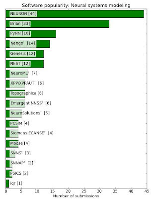
Neuroscience software survey: What is popular, what has problems?

There is an excellent survey on Neuroscience software, carried out by Yaroslav Halchenko and his colleague. Here is the result link: http://neuro.debian.net/survey/2011/results.html
The primary analyses have been published in: Hanke, M. & Halchenko, Y. O. (2011). Neuroscience runs on GNU/Linux. Frontiers in Neuroinformatics, 5:8.

I picked several figures from their result according to my research interests:

ICAtoolbox 3.8 is available now for download

Previously, in my homepage I only provided the content file of the toolbox, and I promised that once I translated the code descriptions into English, I would release it. However, since 2009 when I switched my interest to sparse signal recovery/compressed sensing, I had no time to do the translation job. So I decide to release it now and I apologize for some codes with descriptions/comments written in Chinese. However, if some body has questions, feel free to contact me.

The toolbox can be found in my software page: http://dsp.ucsd.edu/~zhilin/Software.html

PS: Please note that there may be several algorithm codes written by other people. The authors' names are written in the code descriptions.

You can call me "Zorro" instead of "Zhilin" if you like

During my study in US, I find many people don't know how to pronounce my first name "Zhilin", or have difficulty to remember my name. So I decide to give myself a nickname such that people can easily remember or pronounce it. And I choose "Zorro" as my nickname, since I very like Zorro during my childhood and my wife said that I have several obvious characteristics in common with Zorro (except that I don't know how to fight :) ).

Open problems in Bayesian statistics

Mike Jordan wrote a report on his interesting survey on 50 statisticians by asking them what are the open problems in Bayesian statistics. Here is his report:  http://members.bayesian.org/sites/default/files/fm/bulletins/1103.pdf

The top open problems in his report are as follows:

No.1. Model selection and hypothesis testing.

No.2. Computation and statistics.

No.3. Bayesian/frequentist relationships

No.4. Priors

No.5. Nonparametrics and semiparametrics

Andew Gelman made excellent comments on these problems. Here is the link: http://statisticsforum.wordpress.com/2011/04/28/what-are-the-open-problems-in-bayesian-statistics/

Speeding up Latent Dirichlet Allocation (LDA)

Alex has wrote a blog entry on the speed issue of LDA and released his fast LDA algorithm that performs on many computers. Here is the blog entry: http://blog.smola.org/post/6359713161/speeding-up-latent-dirichlet-allocation

In Purdue's MLSS 2011, I was lucky to attend his lectures on graphical models. I like his lectures. The only regret is that I really hope he could give more details on LDA and its variants; for example, giving a detailed development on a variant of LDA models. But I understand the time was limited. After all, the lectures serve for a seminar, not for a college class.

 (Image credit to Alex's Lecture Slides)

Scientific American: How Simple Photos Could Be Used as a Test for a Conscious Machine

The latest issue of Scientific American has an article: How Simple Photos Could Be Used as a Test for a Conscious Machine by  Christof Koch and Giulio Tononi (you need to access the issue to see the full-text. The website just provides you an introduction to the article). It is very interesting. If I have time this summer, I will attend the competition. In fact, I have several ideas to cheat their smart computer. But I don't want to say much right now. However, I'd to say, the picture that the authors provide (see below) is easily recognized by computer algorithms as a unreasonable picture. Their algorithm just needs to do object recognization and then do some semantic reasoning, then it can know this picture is not reasonable. So, don't be misled by the authors' picture.

(The picture's credit to Scientific American)

The T-SBL/T-MSBL paper has been revised

I just uploaded the revised version of the paper "Sparse Signal Recovery with Temporally Correlated Source Vectors Using Sparse Bayesian Learning" accepted by IEEE Journal of Selected Topics in Signal Processing. Several errors in the local analysis have been corrected. This is the final version of the paper.

Misunderstandings on Sparse Bayesian Learning (SBL) for Compressed Sensing (2)

I realized that I've almost forgot to continue this topic. Well, let's continue now. Particularly, I want to put more words on the regularization parameter lambda.

In the first blog entry of this topic (see Misunderstandings on Sparse Bayesian Learning (SBL) for Compressed Sensing (1)), I emphasized that

(1) for a given SBL algorithm, the optimal lambda is different under different experiment settings.
(2) Different SBL algorithms have different optimal lambda under the same experiment settings.
(3) For most SBL algorithms, noise variance is not the optimal lambda value.

Now I'll talk somethings on the lambda learning rules. Generally, most SBL algorithms have their own learning rules for lambda. However, as I emphasized previously, these learning rules basically cannot lead to the best performance for their associated SBL algorithms. To give a clear understanding on this, I'll show you a simulation result below.

The simulation is a comparison of 4 SBL algorithms for the SMV model (single measurement vector case) in a noisy environment (noise variance = 0.01). The 4 SBL algorithms are as follows:
    (1) Wipf & Rao's EM-SBL (published in IEEE TSP, 2004, title: Sparse Bayesian Learning for Basis Selection) using the basic EM updating rule, denoted by EM-SBL
    (2) Qiu & Dogandzic's SBL (published in IEEE TSP, 2010, title: Variance-component based sparse signal reconstruction and model selection), denoted by ExCov
    (3) Ji, Xue & Carin's Bayesian Compressive Sensing (published in IEEE TSP, 2008, title: Bayesian Compressive Sensing), denoted by BCS
    (4) My T-MSBL for the SINGLE measurement vector model (accepted by IEEE Journal of Selected Topics in Signal Processing, 2011, title: Sparse Signal Recovery with Temporally Correlated Source Vectors Using Sparse Bayesian Learning), denoted by T-MSBL for SMV. Although T-MSBL is derived for the MMV cases, it can be also used for SMV cases. In these cases, T-MSBL is essentially the same as EM-SBL, but T-MSBL uses an efficient learning rule for the lambda.
   
First, let's see how the lambda value affects their recovery performance. I plotted their performance as a function of the lambda (Note in SMV cases, EM-SBL and T-MSBL have the same performance curve as a function of lambda), i.e. all the algorithms estimated the solution when fed with a fixed lambda value, and the lambda value varied from 0.001 to 0.33. The performance curve of EM-SBL (T-MSBL for SMV), ExCov, and BCS are plotted as a red solid line, a blue solid line, and a green solid line, respectively, in the following figure.

As we can see, if we can obtain the optimal lambda for each algorithm, then EM-SBL(T-MSBL for SMV) and ExCov have the similar performance, while BCS has the poorest performance. However, if we choose a wrong lambda, say lambda = 0.0381 (this value was calculated according to the suggestion in the Basis Pursuit Denoising paper), then we may conclude that the performance rank is: EM-SBL better than BCS better than ExCov. But if we choose lambda = 0.0042 (this value was calculated according to the suggestion in the BCS code), then we may conclude that the performance rank is: ExCov better than EM-SBL better than BCS. So, unthoughtful choices of lambda may lead to wrong conclusions. Again, we've seen the noise variance (0.01) is not the optimal lambda values of all the SBL algorithms. However, it can be seen as a good estimate for the lambda for ExCov  in this case.

Second, let's see the how lambda learning rules affect the recovery performance. In fact, if we use lambda learning rules to estimate the lambda, we can find the conclusion on performance comparison will change again. I plotted the performance of EM-SBL, ExCov, and my T-MSBL when they used their own lambda leaning rules, shown in red dashed line with square marks, blue dashed line with circle marks, and red dashed line with star marks (for clear display, I omitted the performance of BCS in this case).

You can see, the lambda learning rule of EM-SBL leads to very very poor performance, so poor that even a random guess on lambda may leads to better performance. I've said that in SMV cases the only difference between EM-SBL and T-MSBL is basically the lambda learning rules. Now you can see, the lambda learning rule of my T-MSBL leads to the best performance among the algorithms.

When I read papers in the past one year, I did find that some people heavily relied on the lambda learning rules of SBL. An obvious example is, in terms of recovery performance, SBL algorithms are much better than Lasso, Basis Pursuit, Matching Pursuit etc (this is basically a "truth" well known in our lab). However, in some published simulation results, we found SBL had poorer performance than those algorithms. This is probably due to wrong choices of lambda values, or the use of some lambda learning rules that behaved very poorly.

Here I used the same experiment settings as above to compare the SBL algorithm with Lasso (fed with the optimal regularization value) and Subspace Pursuit (fed with the true number of nonzero elements in the solution vector). Lasso and Subspace Pursuit are plotted as black line with different marks in the following figure:

Clearly, if we allow EM-SBL to use its lambda learning rule, its performance is poorer than Lasso and Subspace Pursuit. However, EM-SBL actually has much better performance than Lasso and Subspace Pursuit, if it uses its optimal lambda value, or uses the noise variance as its lambda value, or uses other lambda values obtained from cross-validation etc.

So, the lambda learning rule is also a crucial factor when evaluating a SBL algorithm's performance. All the lambda learning rules cannot lead to the best performance for their associated SBL algorithms. But some are more effective than others.


Another conclusion is, the work to derive a more effective lambda learning rule is the same valuable as the work to derive a new SBL algorithm using other computation frameworks or models. For example, ExCov is actually an extension of EM-SBL, which treats the nonzero elements of large variance and small variance with different ways. Due to this, the performance curve of ExCov as a function of lambda values is different to that of EM-SBL. When both algorithms choose their optimal lambda value, ExCov has slightly better performance than EM-SBL. However, if both algorithms use their lambda learning rules, ExCov has much better performance than EM-SBL. But if EM-SBL uses the lambda learning rule of T-MSBL (again, note that EM-SBL and T-MSBL is basically the same in SMV cases, except the lambda learning rules), EM-SBL can have better performance than ExCov (see the performance curve denoted by T-MSBL for SMV case). In this sense, it may be better to derive an effective lambda learning rule based on old models than to derive algorithms based on new models.

Actually, lambda learning rules are more important for SBL algorithms in practical applications. This is because in practice, you cannot obtain the optimal lambda value. Although you can use cross-validation, modified L-curve methods or other methods to choose a value for the lambda, for a large-scale dataset, the computational load is heavy.

In simulations you may find some algorithms exhibit excellent performance when use the noise variance as the lambda values, while others behave poorly when use the noise variance as their lambda values. If you conclude that the former algorithms should be better than the latter, you are wrong. This is because it is difficult to accurately estimate the noise variance in practical applications in most cases;  errors in estimating the noise variance cannot be avoided. And you should note that the optimal lambda values of SBL algorithms are not far from each other, and not far from the true noise variance. So, the conclusion you get in simulations when use the true noise variance as the lambda values can be totally different to the conclusion you get in practice when you use the estimated noise variance as the lambda values.

In the next blog entry, I will discuss the issue on the threshold to prune out small gamma_i.

For reproducibility, the experiment settings are as follows:

Gaussian random dictionary matrix of the size 30 x 80
nonzero element number: D = 5
The nonzero elements are generated as: nonzeroW = sign(randn(D,1)).* ( rand(D,1)*0.5 + 0.5 );
And their locations are chosen randomly.
noise variance: 0.01


Reference:

Zhilin Zhang, Bhaskar D. Rao, Clarify Some Issues on the Sparse Bayesian Learning for Sparse Signal Recovery, Technical Report, University of California, San Diego, September, 2011