Is MMV more suitable for dynamic environment (time-varying sparsity) than KF-CS and LS-CS? (3)

Previous experiments are based on the data generated by the file gendata_full.m in the LSCS_KFCS_code.zip. I noted that the data actually are not stable, since the data is generated by the command:
x(:,t) = x(:,t-1) + sqrt(Q1)*randn(m,1);
So, the energy will increase with time. It is interesting to see when the the system x(:,t) is stable (i.e. X(:,t)=P X(:,t) + V, with the eigenvalues of P are less than 1), what's the performance of the algorithms. The stable system is more often encountered in practical problems.

So, I carried out another experiment using stable data. Each coefficient time series was generated as:
x(i,t) = b * x(i,t) + sqrt(1-b^2) * randn(1), with b randomly drawn from [0.7,1).
So, each x(i,:) is a temporally correlated time series.

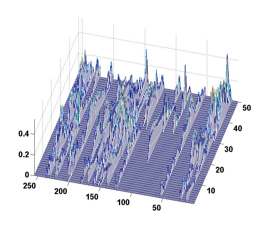
At initial stage, the number of nonzero coefficients were 15. The support of x(:,t) will change at t=15, 25,30. New 10 nonzero coefficient time series were added in the support at t=15 and 30, while 4 existing coefficient time series were removed at t=25.

A picture of the evolution of coefficient amplitude is given below (the label for the bottom axis is the index of coefficient; the label for the right axis is the snapshot index; the label for the left axis is the absolute amplitude):

The dictionary matrix was 60 by 256. The total number of snapshot was 50. Noise standard variance was 0.01 (about 20 dB). I compared KF-CS, M-SBL and my T-MSBL. KF-CS was performed on the whole data. T-MSBL and M-SBL was performed on 5 segments (I evenly divided the whole data into 5 short segments with 10 snapshots). Experiment was repeated for 25 trials. Here is the result:

We can see T-MSBL achieved the best performance. I am somewhat surprised by the behavior of KF-CS. Probably KF-CS's detection to disappearing coefficients is more sensitive to the pre-defined values. As for elapse time, KF-CS cost about 190 second, while T-MSBL and M-SBL cost about 3 seconds (note here the input argument MIN_GAMMA for the SBL algorithms was set to 1e-3, which was different to the values in previous experiments. Different values of  this input argument can result in significant change in speed).

The strange behavior of KF-CS in above experiment is probably due to the algorithm sensitive to the pre-defined threshold to remove disappearing coefficients. I used the threshold value given by the code, but didn't try other various values, because each running took much time. So, to remove the effect of this issue, I designed another experiment.

The experiment is an exactly MMV experiment, i.e. the support of each column in X didn't change (all satisfy the common sparsity assumption). Here is the result:

As in the above experiment, T-MSBL and MSBL were performed on 5 segments. And their final results were the concatenation of the recovered results from each segment. Again, we obtain the same conclusion.

So, I believe, for time-varying sparsity problems, dividing the whole data into several short segments and then using MMV algorithms on each segment is an effective method.

Referece:
Z. Zhang, B.D.Rao, Exploiting Correlation in Sparse Signal Recovery Problems: Multiple Measurement Vectors, Block Sparsity, and Time-Varying Sparsity, ICML 2011 Workshop on Structured Sparsity


-----
Another tulip is flowering in my patio:

Is MMV more suitable for dynamic environment (time-varying sparsity) than KF-CS and LS-CS? (2)

As I said in the previous post, MMV algorithms can be used to dynamical environment (i.e. the problem with time-varying sparse patterns). In the experiment of that post, I used M-SBL as an example (other MMV algorithms can be used also). It was performed on the whole data (Time 0 to Time 60). Here I gave another experiment, in which I segmented the whole data into 6 shorter segments and then performed MSBL on each segment (i.e. step by 10 snapshots), and finally concatenated the recovered data from each segment.

Here is the result (click the picture for large view):

The pink dashed line is the performance curve of the method. The errors in the first few snapshots are obviously reduced, compared to the performance curve of the method that performing MSBL on the whole data (indicated by the red solid line).

Obviously, MMV algorithms can be applied to dynamic compressed sensing problems in this block on-line style. In the above experiment MSBL stepped by 10 snapshots. Here are more experiment results when MSBL stepped by 2, 3 and 5 snapshots (for comparison, I also plotted the results of KF-CS,KF-Genie, LS-CS, and MSBL applied on the whole data from the above experiment):

 

Referece:

Z. Zhang, B.D.Rao, Exploiting Correlation in Sparse Signal Recovery Problems: Multiple Measurement Vectors, Block Sparsity, and Time-Varying Sparsity, ICML 2011 Workshop on Structured Sparsity

Do a cognitive neuroscience experiment on myself

Plasticity is an amazing ability of brains. Since today I will start a cognitive neuroscience experiment on myself and the experiment will last for at least one month. I don't want to tell details of the experiment right now. But if I success, I will describe the amazing experiment here. Let's see......



btw: Today my Nepenthes aristolochioides opened another new pitcher. This species is well-known for its 'beehive' shaped pitchers. Here is the picture:

Is MMV more suitable for dynamic environment (time-varying sparsity) than KF-CS and LS-CS? (1)

It is viewed that the MMV model is an special case of the dynamic sparse model, and thus some people probably believe that algorithms for the MMV model may not be suitable for the dynamic sparse model. Here I'll give an experiment to show that it is not the case. It is more probably that algorithms for the MMV model is more suitable for the dynamic sparse model.

First, I'll give the necessary background on the two models.

The MMV model (i.e. multiple measurement vector model) is an extension of the basic compressed sensing model. It is expressed as:
Y = AX + V,
where Y is the N by L measurement matrix (known), A is the N by M dictionary matrix (known), and X is the unknown M by L coefficient matrix (unknown). V is the unknown noise matrix. Clearly, when L=1, the model is the basic compressed sensing model (the model from which the Lasso, Basis Pursuit, Matching Pursuit and other numerous algorithms were derived). In the MMV model, a key assumption is that there are few nonzero rows in X (i.e.  the common sparsity assumption). It is worthy mentioning that under mild conditions algorithms' recovery performance is exponentially increased with increasing L (i.e. the number of measurement vectors). And in many applications (such as MRI image series processing, Source localization, etc) we can always obtain several or many measurement vectors. Many algorithms have been proposed, such as M-SBL [1] (assuming each row in X has no temporal correlation) and T-SBL/T-MSBL [2] (assuming each row in X could have temporal correlation).

However, in applications we cannot ensure all the column vectors in X have the same support (i.e. indexes of the nonzero elements in a column vector). It is more probably that the support of columns is slowly changing, i.e. the columns in X have time-varying sparsity patterns. This model is generally called the dynamic sparse model. Several algorithms have been proposed, such as the Kalman Filtered Based Compressed Sensing (KF-CS) [3], Least-Square Compressed Sensing (LS-CS) [4], and the algorithm based on Belief Propagation [5].

Since the common sparsity assumption in the MMV model is not satisfied in the dynamic sparse model, one may think that algorithms derived in the MMV model may not be suitable for the dynamic sparse model. However, as long as the number of total nonzero rows in X is not too many (e.g. less than (N+L)/2 [6]), MMV algorithms can be used for the dynamic sparse model, and even have better performance.

Here is an experiment, which compares the M-SBL,  KF-CS and LS-CS. The simulation data and the KF-CS and LS-CS codes all come from the author's website: http://home.engineering.iastate.edu/~namrata/research/LSCS_KFCS_code.zip. The M-SBL code comes from my website: http://dsp.ucsd.edu/~zhilin/ARSBL_1p2.zip.

I directly used the data generated by the m-file: runsims_final.m in the LSCS_KFCS_code.zip downloaded via the above link,  and used the original matlab command to call KF-CS and LS-CS algorithms, i.e:
[x_upd,T_hat] = kfcs_full(y,Pi0,A,Q,R)
[x_upd_lscs,T_hat_lscs,x_upd_csres] = lscs_full(y,Pi0,A,Q,R);
This commands were given by the author. I didn't change anything.

The command to call M-SBL is given by:
[x_sbl,gamma,gamma_used,k] = MSBL(A, y, R(1,1), 0, 1e-4, 1000, 0);

Experiment was repeated for 63  trials. The averaged results (from Time 0 to Time 60) are shown in the following pic (click the pic for large view):

Here we can see, both KF-CS  and LS-CS have large errors when the sparsity profile of the columns in X changes (indicated by the four large bumps). In contrast, M-SBL does not have this phenomenon and has much small errors in most duration. KF-Genie indicates the Kalman-Filter estimation when the support of each column in X is known.

The averaged elapse time is (in my notebook):
KF-CS is 168.5 seconds
LS-CS is 168.3 seconds
M-SBL is  19.7 second

I have to emphasize, if we segment the whole data into several shorter segments, and then perform M-SBL on each segment and concatenate the results from each segment, we can get better performance.

So, the conclusion is, the MMV model has great potential for the problem of time-varying sparsity patterns. This is somewhat like that people generally view each short segment of a nonstationary signal as a stationary signal. So, viewing a time-varying sparsity model as concatenation of several MMV models is probably a better way to solve the time-varying sparsity model.

Some of the results can be found in [7].

Reference:

[1] D.P. Wipf and B.D. Rao, An Empirical Bayesian Strategy for Solving the Simultaneous Sparse Approximation Problem, IEEE Transactions on Signal Processing, vol. 55, no. 7, July 2007

[2] Z.Zhang, B.D.Rao, Sparse Signal Recovery with Temporally Correlated Source Vectors Using Sparse Bayesian Learning, accepted by IEEE Journal of Selected Topics in Signal Processing, [arXiv:1102.3949]

[3] Namrata Vaswani, Kalman Filtered Compressed Sensing, IEEE Intl. Conf. Image Proc. (ICIP), 2008

[4] Namrata Vaswani, "LS-CS-residual (LS-CS): Compressive Sensing on the Least Squares Residual", IEEE Trans. Signal Processing, August 2010

[5] J.Ziniel, L.C.Potter, P.Schniter, Tracking and smoothing of time-varying sparse signals via approximate belief propagation, Asilomar 2010

[6] SF Cotter, BD Rao, Sparse solutions to linear inverse problems with multiple measurement vectors, IEEE Trans. on Signal Processing, 2005

[7] Z. Zhang, B.D.Rao, Exploiting Correlation in Sparse Signal Recovery Problems: Multiple Measurement Vectors, Block Sparsity, and Time-Varying Sparsity, ICML 2011 Workshop on Structured Sparsity

Research Tips From Dr. Bai Lu

Here are some research tips given by Dr. Bai Lu when he gave a talk in China several years ago. Very helpful for young researchers such as me. In fact, life is too short to do trivial/normal research.

Two misunderstandings:

(1) No body did this ---> I should do this

(2) This is new  ---> This is good

What is a first-class paper/research?

(1) Major advance in a classic field

(2) New techniques and methods that can be widely used

(3) Discoveries with obvious practical implications

(4) Conceptual breakthrough, novel ideas

(5) Challenge to traditional views, break dogma

(6) Opening up new area, cross board

What is a mediocre paper/research?

(1) Horizontal growth (e.g. I made the discovery in rats, you find the same in cat)

(2) Filling gaps (e.g. A actives B which is known to induce C. You show that A enhances C)

(3) Working out details

(4) Support existing idea, "me too"

(5) Follow up

(6) Incomplete study, preliminary

Professor Terrence Sejnowski elected to National Academy of Engineering

Recently, there is a cool news on Professor Terry, a professor of UCSD and Salk Institute. I once took his class and was impressed by his super-clear thinking and vision. Prof. Terry is the head of the Institute of Neural Computation, which has many research institutes/labs. The Swartz Center for Computational Neuroscience, famous for applying ICA to EEG analysis and led by Prof. Scott, is one of them.


February 08, 2011 (The news comes from: http://www.salk.edu/news/pressrelease_details.php?press_id=468)

LA JOLLA, CA—Salk Institute professor Terry J. Sejnowski, Ph.D., has been elected a member of the National Academy of Engineering, an honor considered one of the highest accolades in the engineering world. Dr. Sejnowski, whose work on neural networks helped spark the neural networks revolution in computing in the 1980s, is recognized for his "contributions to artificial and real neural network algorithms and applying signal processing models to neuroscience."
 
Dr. Sejnowski is also a member of the National Academy of Sciences and the Institute of Medicine, making him one of only ten living individuals to have been elected to all three branches of the National Academies.


"Terry is a truly visionary scientist," said Salk president William R. Brody. "He was the first one to apply the power of computing to the brain, pioneering the field of computational neuroscience. It's a beautiful example of how transcending disciplines can revolutionize science and open up entirely new fields of study. We are very proud of what Terry and his students have accomplished."

Dr. Sejnowski, a Howard Hughes Medical Institute investigator and head of the Computational Neurobiology Laboratory, studies real neural networks in which the interaction of many neurons produces surprisingly complex behavior, and he has also shown how artificial neural networks can solve practical engineering problems.

A physicist by training, he combines both experimental and modeling techniques, habitually overthrowing scientific dogma. For decades the assumption was that the most important information from neurons was the total number of times the neurons fired. Dr. Sejnowski, however, discovered that the timing and pattern of nerve impulses is just as important for understanding brain function. Similarly, he demonstrated that the release of chemical signals from nerves isn't restricted to synapses, as neuroscientists had previously believed, but takes place outside the expected region.

He has created computer models of networks of neurons to explore the mechanisms underlying attention in the awake brain and brain rhythms in the sleeping brain and the links between them. These models also help explain how epilepsy arises from imbalances in brain circuits.

By studying how computer simulations can perform operations that resemble the activities of the cerebral cortex, Dr. Sejnowski hopes to gain new knowledge of how the human brain is capable of learning and storing memories. This knowledge ultimately may provide medical specialists with critical clues to combating schizophrenia and other disorders that rob people of their critical thinking ability and memory for faces, names, places and events.

Dr. Sejnowski joins Dr. Irwin Jacobs, chair of the Salk Board of Trustees, and Dr. William Brody as the third member of the National Academy of Engineering at the Salk Institute.

About Terrence J. Sejnowski:
Dr. Sejnowski graduated from Case Western Reserve University and earned his doctorate in physics at Princeton University. After completing postdoctoral research studies in biology at Princeton and in neurobiology at Harvard University, he held an appointment in the department of biophysics at Johns Hopkins University before he was appointed a professor in the Department of Biological Sciences at the University of California, San Diego. In 1988, he joined the Salk Institute for Biological Studies, where he directs the Crick-Jacobs Center for Computational Neurobiology. He also heads the Institute for Neural Computation and co-directs the NSF Science of Learning Center, both at UCSD.
In addition to being a member of the National Academy of Engineering, Dr. Sejnowski is a member of the Institute of Medicine and the National Academy of Sciences and has been the recipient of multiple honors, including the Wright Prize for interdisciplinary research from Harvey Mudd College, the Hebb Prize and the Neural Network Pioneer Award from the Institute of Electrical and Electronics Engineers. He has published over 300 scientific papers and 12 books, including The Computational Brain, with UC San Diego professor of philosophy Patricia Churchland.

Misunderstandings on Sparse Bayesian Learning (SBL) for Compressed Sensing (1)

I will gradually discuss some misunderstandings on the sparse Bayesian learning (SBL), which I have seen in some published papers.

One misunderstanding is the "noise variance" term (written in $\lambda$ or $\sigma^2$ in the literature on SBL). From the Bayesian view, it seems OK to view $\lambda$ as the noise variance. And hence, in computer simulations, people think that setting $\lambda$ to be the true noise variance can allow SBL algorithms to reach their full strength for compressed sensing, and thus this strategy is fair to SBL algorithms when doing performance comparison.

But I have to say, for SBL algorithms the optimal value for $\lambda$ is not the true noise variance, and thus some performance comparisons are not correct!

Here I show some simple experiment results. We can see the optimal value for $\lambda$ is generally larger than the true noise variance.

I use the M-SBL algorithm proposed by David in 2007. The code can be downloaded from the link. Note that this code is a modified version of David's code, since some parameter settings in the latter code are not suitable for performance comparison in low SNR cases.

The Gaussian dictionary matrix was of size 40 by 120 (i.e. N=40, M=120). The number of measurement vectors, L, was 3. The true noise variance was 0.01 (The SNR was around 10dB). The number of nonzero rows in the source matrix (or called the coefficient matrix, the solution matrix), K, was set to be 4, 12, and 16. For each different K, the experiment was repeated 200 times. In each trial, the M-SBL algorithm was fed with different values of $\lambda$. Its performance was measured by two measures: the failure rate and the mean square error (MSE). The failure rate is defined in David's M-SBL paper. These are general experiment settings, for detailed description of the experiments, one can see my paper.

Here is the result (click the figure for full view):

From the figure, we can draw the following conclusions:

(1) The optimal value of $\lambda$ is not equal to the true noise variance. The optimal value is larger than the true noise variance.

(2) Different measures correspond to different optimal values (or different ranges of optimal values). In other words, for given experiment settings, the optimal value for $\lambda$ in terms of MSE is different to the optimal one in terms of the failure rate. This observation is more obvious when using my T-SBL/T-MSBL. 

(3) Changing any experiment setting (e.g. K, L, N, M), the optimal value will accordingly change (in the above experiment, I changed the K). For example, in the figure we can see: with K (the number of nonzero rows in the coefficient matrix) increasing, the optimal value is decreasing, but still larger than the true noise variance.

In fact, I have to add the fourth conclusion (although I don't show here):

(4) For different SBL algorithms, the optimal values for $\lambda$ are different.

Based on these conclusions, now we know that the strategy of setting $\lambda$ being the true noise variance is problematic in algorithm comparison. Suppose we compare two SBL algorithms, say SBL (I) and SBL (II). And suppose that for given experiment settings,  the optimal $\lambda$ of SBL (I) is much closer to the true noise variance than the one of SBL (II). Then, when we set the $\lambda$ to be the true noise variance for the two algorithms, SBL (I) most likely shows better performance than SBL (II), although SBL (II) actually has better performance than SBL (I) if both the two algorithms choose their optimal $\lambda$ values.

Another lesson from the experiment is: when changing any experiment setting, we should again find the optimal $\lambda$ value; otherwise, we can get wrong conclusion. For example, in the above experiment, if we fixed $\lambda$ to be the true noise variance (0.01), we could find that the algorithm's MSE at K=4 is even larger than the MSE at K=12 ! (note that the smaller the K is, the easier the inverse problem is).

Now I think you've believed how important to choose the optimal $\lambda$ in performance comparison.  Especially, when two algorithms have very close performance curves, you must be very cautious to avoid the above wrong strategies.

NOTE: The above conclusions and lessons not only are applied to the comparison of SBL algorithms, but also are applied to the comparison of SBL algorithms to non-SBL algorithms, and also are applied to the comparison of non-SBL algorithms (the regularization parameters of $\ell_1$ algorithms exist similar phenomena!).

You may ask: although the optimal values of $\lambda$ are important, in practice we probably have no way to find them. Yes, you are right. The above conclusions and lessons should be kept in mind when people are really care about which one is better than which one. But in practice, you can use some widely used methods to choose a sub-optimal value for $\lambda$ and do performance comparison. But in this case, you need to be very careful about your conclusions. At least, you cannot say, algorithm (I) is better than algorithm (II). You need to emphasis that when using your $\lambda$ setting strategy, algorithm (I) shows better performance than algorithm (II), and keep in mind that your reader may draw the opposite conclusion when using his/her own strategy for finding a sub(optimal) value for $\lambda$.

The fact that the optimal $\lambda$ is not equal to the true noise variance should not be surprising. In fact, $\lambda$ can be interpreted as noise variance is only reasonable when the dictionary matrix is not underdetermined.

Similarly,  the matrix B in my T-SBL/T-MSBL algorithms cannot be simply interpreted as the covariance matrix of sources. And one should not be surprised that using a single matrix B can lead to excellent performance even if different sources have different temporal correlations.


Reference:

Zhilin Zhang, Bhaskar D. Rao, Clarify Some Issues on the Sparse Bayesian Learning for Sparse Signal Recovery, Technical Report, University of California, San Diego, September, 2011

Losing sleep is a big problem for me when I get excited in my research

Again, I lost sleep tonight. I have many things to do, many thoughts to organize, and many papers to write down. I couldn't stop my brain thinking.

Just now I remembered a saying: if you love a person, ask him/her to do research; if you hate a person, also ask him/her to do research.

Yes, research is such a magic thing making people like me forget eating and losing sleep.

M-SBL Using Gaussian Scale Mixture Model ?

Recently, there are some interesting works that use the Gaussian scale mixture (GSM) model in the framework of sparse Bayesian learning (SBL) . But I have not seen any papers using this model to modify the original MSBL algorithm proposed by David, or to deal with the multiple measurement vector (MMV) model under the common sparsity assumption, the model that was proposed by Cotter & Rao (Although there are some papers considering MMV models, their models are different to here). It seems that the GSM model can model the spatial dependency in X in some degree. So, to satisfy my curiosity, I modified the David's MSBL using the GSM model.

The MMV model under the common sparsity assumption is given by:
Y=AX + V,
where Y is the available data matrix of size N x L, A is the known dictionary matrix, and X is the unknown solution matrix of size M x L. V is the noise matrix. Assume:
X_i = sqrt(z) U_i,    i=1,...,L,
where X_i is the i-th column of the solution matrix X, z is a positive scalar, U_i is a column vector with elements being independent. Each element of U_i satisfied a Gaussian distribution N(0,\gamma_i). Then, following the steps of the derivation of MSBL, we can easily obtain the GSM based MSBL algorithm.

The algorithm has the similar form to MSBL. Essentially, their only difference is that the $\lambda$ in MSBL becomes $\lambda / z $ in GSM-MSBL. So, it seems that GSM-MSBL may correct the learning of $\lambda$. It is known that SBL's learning rules for $\lambda$ are not robust in low SNR cases. So, I expect that GSM-MSBL can yield a better recovery performance than MSBL through the correction of the learning rule for $\lambda$.

However,  by observing the derived learning rule for z, i.e.

I found the learning rule is exactly equal to 1, i.e. z = 1! In this case, GSM-MSBL is the same to MSBL. Admittedly, the above learning rule is obtained from the data using the empirical Bayesian method. Maybe there exist other methods to estimate z. But currently I don't know.

If anybody has got a GSM based MSBL algorithm showing better performance, please let me know.

Answer Bob's question on the paper: Sparse Signal Recovery with Temporally Correlated Source Vectors Using Sparse Bayesian Learning

Today I received an email from a reader, Bob, asking me why in high SNR cases or noiseless cases T-MSBL is better than T-SBL. What confused Bob is that in the paper T-MSBL is an approximation to T-SBL (using the approximation (20)). Both of them, in theory, are identical in the noiseless cases or the correlation-free cases. So, by intuition, T-MSBL should not be better than T-SBL, and in noiseless cases or correlation-free cases, T-MSBL has the same performance to T-SBL.

Thanks Bob for the good question.

First, I have to say, there is a slight difference between T-MSBL and T-SBL in noiseless cases or correlation-free cases. For T-SBL, the learning rule for B is given by Equation (13). For T-MSBL, the learning rule is given by Equation (28)-(29), which cannot be obtained from (13) using the approximation (20). As I stated in my paper, different B's can result in different performance. But I guess if T-MSBL adopts the rule (27), instead of (28)-(29), it should have the same performance to T-SBL in noiseless cases or correlation-free cases (because (27) is the simplified version of (13)).

Sparse Signal Recovery with Temporally Correlated Source Vectors Using Sparse Bayesian Learning

Finally, I finished the revise of this paper, which was submitted to IEEE Journal of Selected Topics in Signal Processing for the second-round review. The paper can be downloaded from my homepage or from http://arxiv.org/abs/1102.3949

This paper addressed a problem in the multiple measurement vector (MMV) model in compressed sensing. For the MMV model, i.e.
Y=AX + V,
most algorithms apply Lq norm on the rows of the solution matrix X, while apply Lp norm on the evaluated values of the row norms. For example, the MMV extension of the classic Basis Pursuit uses the L2 norm to evaluate each row of X, while uses the L1 norm to constrain the row sparsity of X. In fact, most algorithms uses the L2 norm or the L_infinity norm to evaluate the rows of X. Clearly, these norm operations are blind to data structures, i.e. the correlations of elements in each nonzero row of X. I call this temporal correlation (this term is to emphasize the difference from those considering the correlations among different rows --- which are called spatial correlation in many literature). In this paper, by deriving two sparse Bayesian learning algorithms, I showed that algorithms can get  improved recovery performance if we replace the Lq norm imposed on each row with the Mahalanobis distance measure. Actually, the improvement is very surprising, as the experiments of the paper showed.

However, the development of new algorithms is just a part of the story. Computer simulations have found some interesting phenomena of the algorithms.

First, let me ask you a question:

When the temporal correlations exist, say with correlation coefficient being 0.9, does the recovery performance of algorithms become worse? 

It seems that the answer is YES, because one may intuitively think that when the temporal correlations exist, each individual solution vector (i.e. Xi, with [X1,..., X_L]=X ) provides less information about the locations of nonzero rows. For example, consider an extreme case: suppose the temporal correlation coefficients are 0.999999. In this case, each individual solution vector Xi (i=1,...,L) is almost the same. Consequently, algorithms' performance is very close to their performance when only one measurement vector is available, namely, L=1 (let's consider a noiseless environment for simplicity).

However, my paper showed that the answer is NO. Here is one experiment result:

This is Fig.7 in my paper. M/N is the ratio of column number over row number of the dictionary matrix. T-MSBL is one of my derived algorithms, which exploits temporal correlations. MSBL is a benchmark algorithm proposed by David Wipf in 2007. $\beta$ indicates the temporal correlations. The relation of MSBL's performance to the temporal correlations is expected by our intuition: the higher the temporal correlations are, the worse the performance is. However, one can see the T-MSBL's performance becomes better with higher temporal correlations.

Next, let's see another extreme experiment. In this experiment (noiseless), the temporal correlations  approximate to 1 or -1 infinitely (temporal correlation is given by $\beta = sign(C)(1-10^{-|C|})$ ). Just imaging what's the value when C=10 and what this means how similarity among individual solution vectors! However, from the figure below, we again see the different behaviors of T-MSBL and MSBL. For MSBL, when |C| becomes large, its performance is close to its performance in the case of L=1. In contrast, T-MSBL still keeps the same performance, no matter how large |C| is.

As a reminder, the high temporal correlations indicate the ill-condition of the solution matrix X.

The two experiments clearly showed the importance of exploiting temporal correlations among different solution vectors, which is largely ignored in the field of compressed sensing. Up to now I've not found any existing algorithms have the similar performance to my T-MSBL and T-SBL. Also, I didn't find any theories can explain the behaviors of T-MSBL/T-SBL in the above two figures. If you find any algorithms with the similar performance, or find any theories can explain these phenomena, please let me know.

The third point that I want to emphasize is: I strongly suggest the use of Mahalanobis distance measure instead of the Lq norms imposed on the nonzero rows of X. We have seen lots of works (both theoretical and algorithmic) to analyze the benefits from the Lq norms, such as the L2 norm or the L_infinity norm. However, these data-structure blind norms cannot lead to satisfying performance in some practical applications, since practical signals or image sequences generally have strong temporal correlations. At least, using Mahalanobis distance measure can lead to better performance. But I have to admit, this work is just a start-point. Further study is needed.