My blogs reporting quantitative financial analysis, artificial intelligence for stock investment & trading, and latest progress in signal processing and machine learning

Monday, May 23, 2011

New Versions of T-MSBL/T-SBL are Available for Download

Finally, I almost re-coded the two algorithms for convenient use. The main feature of the new versions  is, for general users who don't know much about SBL and don't want to tune parameters, they just need to type the command:

X_est = TMSBL(Phi, Y); % for most noisy cases (SNR from 7-23dB)

or according to your rough guess about the SNR, type the command:

X_est = TMSBL(Phi, Y, 'noise', 'large');  % for SNR < 7dB
X_est = TMSBL(Phi, Y, 'noise', 'mild') ;  % for SNR from 7-23dB
X_est = TMSBL(Phi, Y, 'noise', 'small') ; % for SNR > 23dB
X_est = TMSBL(Phi, Y, 'noise', 'no') ;      % no noise

Each command uses a set of pre-defined parameter values, which probably are suitable for most compressed sensing experiments. But they may not be optimal for your specific task. For example, if the row-norms of your X are very small or very large, you may need to change the input argument 'prune_gamma'. Please read the demo files to see the experiment settings. If you want to get the best performance for your task, you can read my suggestions on tuning parameters from the cookbook: http://sccn.ucsd.edu/%7Ezhang/TSBL_cookbook.pdf. I strongly suggest everyone to read the short cookbook before using the codes.

The codes can be downloaded at: https://sites.google.com/site/researchbyzhang/t-msbl


If you have any questions or suggestions, please feel free to contact me. And, if you find the codes do not perform well, please let me know.


==========================================
There are two pictures of my plants in that cookbook. Interesting, right? Just relax :)
It is called cobra plant, because it is like a cobra :)

Another one is called N. ampullaria (red) x N. sibuyanensis. It is a nepenthes.


Saturday, May 21, 2011

Codes of T-SBL and T-MSBL are under updating

I just found there are two bugs in the codes of T-SBL and T-MSBL for high SNR cases or noiseless cases. I am now correcting them. Also, I realized that probably some users dislike setting these input arguments; they want to just input the dictionary matrix Phi and the measurement data Y, then wait for the results. So, I'm trying to simplify the setting of input arguments.

Please give me one more day. I will upload the codes again in this weekend.

Thursday, May 19, 2011

Life Without Limits, No Arms, No Limbs and No Worries

Today I watched a video from Youtube. It is a talk by Nick Vujicic. It's really a wonderful video. Anyone who is in depression or feel hopeless should watch this inspirational video. Anybody who has arms and legs has no reason to give up in life.


He has a book titled :

Life Without Limits: Inspiration for a Ridiculously Good Life

can be bought from Amazon. DVD is also available at Amazon.

Codes of T-SBL and T-MSBL are available

I have posted the codes of T-SBL and T-MSBL on my homepage, which are developed in my paper:

Zhilin Zhang, Bhaskar D. Rao, Sparse Signal Recovery with Temporally Correlated Source Vectors Using Sparse Bayesian Learning, IEEE Journal of Selected Topics in Signal Processing, Special Issue on Adaptive Sparse Representation of Data and Applications in Signal and Image Processing, 2011, accepted.

They can be downloaded from here. But before you running/testing the codes, I strongly suggest you spend 3 minutes in reading the short cookbook on how to set suitable input parameters. There are four study cases, such as noiseless case, mild noisy case, strongly noisy case, and so on. You can check the example in each case for advice on choosing parameters. But don't be scared. Generally, in any case you only need to set 1 or 2 parameters, and setting them is a piece of cake (you do not need to understand SBL or read any SBL paper!)

Along with the codes of T-SBL and T-MSBL, there are several demos, which can re-produce the experiment results in my paper.

The paper has been revised. But it is still not the final version. I am now revising the language :( The final version will be uploaded at the end of this month).

Also, I've uploaded the code of M-SBL. It can be downloaded from here. Yes, David has a code of M-SBL. But his code is not suitable for noisy cases and even not suitable for noiseless case. I also suggest you to read the comments in my code to correctly use M-SBL for algorithm comparison.

Saturday, May 14, 2011

Insights from T-SBL/T-MSBL

Recently I have two papers that reveal something interesting from T-SBL/T-MSBL. They are:

[1] Z.Zhang, B.D.Rao, Iterative Reweighted Algorithms for Sparse Signal Recovery with Temporally Correlated Source Vectors, ICASSP 2011Downloaded here

[2] Z.Zhang, B.D.Rao, Exploiting Correlation in Sparse Signal Recovery Problems: Multiple Measurement Vectors, Block Sparsity, and Time-Varying Sparsity, ICML 2011 Workshop on Structured Sparsity: Learning and Inference. Downloaded here
(Thank Igor for highlighting this paper in his blog Nuit Blanche)

 [1] gave the iterative reweighted L2 version of T-SBL/T-MSBL. The most interesting thing is, this insight motivated us to modify most existing iterative reweighted L2 algorithms for better performance in the presence of temporally correlated source vectors. Yes, I mean "most existing iterative reweighted L2 algorithms". Although the paper only gave two examples, I indeed have modified other famous reweighted L2 algorithms, such as the Daubechies's algorithm.

[2] gave the iterative reweighted L1 version of T-SBL/T-MSBL (of course, there are other interesting stuff in [2]). And, similarly, this motivated us to modify existing iterative reweighted L1 algorithms, such as the group Lasso (note that group Lasso can be applied on the MMV model).

The key idea is (I have emphasized this many times in my blog): replacing the Lq norm (such as L2 norm, L_infinity norm) imposed on the rows of the solution matrix by the Mahalanobis distance measure, i.e.:

Of course, the matrix B needs to learn adaptively from the data. However, in some cases you can pre-define it before runing algorithms.

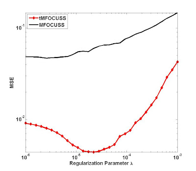
Here is an example (taken from [1]) showing how to modify the M-FOCUSS algorithm (a typical iterative reweighted L2 algorithm).

The original M-FOCUSS is given by:

We just simply replace the L2 norm indicated by the red circle with the Mahalnobis distance measure, obtaining:
The learning rule for the matrix B is similar to the one in T-MSBL. See [1] for details. Let's see what happen to the performance.

Here is a simulation: The Gaussian dictionary matrix was of the size 50 x 200. The number of nonzero rows in the solution matrix was 20. The temporal correlation of each nonzero row was 0.9. The number of measurement vectors was 4. Noise standard variance was 0.01. To avoid the disturbance of incorrect choosing the regularization parameter \lambda, we chosen 30 candidate values for \lambda, and for each value we ran the original MFOCUSS and the new tMFOCUSS for 300 trials. The averaged performance as a function of \lambda was given below:


See the improvement? Funny, ha!

The codes of tMFOCUSS and the the simulation can be downloaded from my website: https://sites.google.com/site/researchbyzhang/software

Other examples can be found in my paper [1].


Well, now let's go to the stuff on iterative reweighted L1 algorithms for the MMV model. The framework of reweighted L1 is given by:
where its weights are:

Now, we replace the Lq norm in the weights by the Mahalanobis distance measure, obtaining:

An noiseless simulation was carried out (see [2] for details). The temporal correlation of each row of the solution matrix was 0.9. The matrix B can be learned using the rule given in the paper. But here it was set to the true value. The result is shown below:


Not surprising, we see the improvement! But I have to say, in this case, we may have to solve a non-convex problem.

Interesting, right? Why not to modify your favorite reweighted L1 algorithms or L2 algorithms to improve their performance in the presence of temporally correlated source vectors? You should know, in practice, we often encounter the cases when the source vectors are correlated (In EEG/ERP source localization, the correlation could be larger than 0.95!).

But note, for some algorithms, improvement by the straightforward modification may be not obvious -- There is no free-lunch!