My blogs reporting quantitative financial analysis, artificial intelligence for stock investment & trading, and latest progress in signal processing and machine learning

Monday, April 18, 2011

Is MMV more suitable for dynamic environment (time-varying sparsity) than KF-CS and LS-CS? (3)

Previous experiments are based on the data generated by the file gendata_full.m in the LSCS_KFCS_code.zip. I noted that the data actually are not stable, since the data is generated by the command:
x(:,t) = x(:,t-1) + sqrt(Q1)*randn(m,1);
So, the energy will increase with time. It is interesting to see when the the system x(:,t) is stable (i.e. X(:,t)=P X(:,t) + V, with the eigenvalues of P are less than 1), what's the performance of the algorithms. The stable system is more often encountered in practical problems.

So, I carried out another experiment using stable data. Each coefficient time series was generated as:
x(i,t) = b * x(i,t) + sqrt(1-b^2) * randn(1), with b randomly drawn from [0.7,1).
So, each x(i,:) is a temporally correlated time series.

At initial stage, the number of nonzero coefficients were 15. The support of x(:,t) will change at t=15, 25,30. New 10 nonzero coefficient time series were added in the support at t=15 and 30, while 4 existing coefficient time series were removed at t=25.

A picture of the evolution of coefficient amplitude is given below (the label for the bottom axis is the index of coefficient; the label for the right axis is the snapshot index; the label for the left axis is the absolute amplitude):
The dictionary matrix was 60 by 256. The total number of snapshot was 50. Noise standard variance was 0.01 (about 20 dB). I compared KF-CS, M-SBL and my T-MSBL. KF-CS was performed on the whole data. T-MSBL and M-SBL was performed on 5 segments (I evenly divided the whole data into 5 short segments with 10 snapshots). Experiment was repeated for 25 trials. Here is the result:

We can see T-MSBL achieved the best performance. I am somewhat surprised by the behavior of KF-CS. Probably KF-CS's detection to disappearing coefficients is more sensitive to the pre-defined values. As for elapse time, KF-CS cost about 190 second, while T-MSBL and M-SBL cost about 3 seconds (note here the input argument MIN_GAMMA for the SBL algorithms was set to 1e-3, which was different to the values in previous experiments. Different values of  this input argument can result in significant change in speed).

The strange behavior of KF-CS in above experiment is probably due to the algorithm sensitive to the pre-defined threshold to remove disappearing coefficients. I used the threshold value given by the code, but didn't try other various values, because each running took much time. So, to remove the effect of this issue, I designed another experiment.

The experiment is an exactly MMV experiment, i.e. the support of each column in X didn't change (all satisfy the common sparsity assumption). Here is the result:

As in the above experiment, T-MSBL and MSBL were performed on 5 segments. And their final results were the concatenation of the recovered results from each segment. Again, we obtain the same conclusion.

So, I believe, for time-varying sparsity problems, dividing the whole data into several short segments and then using MMV algorithms on each segment is an effective method.

Referece:
Z. Zhang, B.D.Rao, Exploiting Correlation in Sparse Signal Recovery Problems: Multiple Measurement Vectors, Block Sparsity, and Time-Varying Sparsity, ICML 2011 Workshop on Structured Sparsity


-----
Another tulip is flowering in my patio:

Sunday, April 17, 2011

Is MMV more suitable for dynamic environment (time-varying sparsity) than KF-CS and LS-CS? (2)

As I said in the previous post, MMV algorithms can be used to dynamical environment (i.e. the problem with time-varying sparse patterns). In the experiment of that post, I used M-SBL as an example (other MMV algorithms can be used also). It was performed on the whole data (Time 0 to Time 60). Here I gave another experiment, in which I segmented the whole data into 6 shorter segments and then performed MSBL on each segment (i.e. step by 10 snapshots), and finally concatenated the recovered data from each segment.

Here is the result (click the picture for large view):


The pink dashed line is the performance curve of the method. The errors in the first few snapshots are obviously reduced, compared to the performance curve of the method that performing MSBL on the whole data (indicated by the red solid line).

Obviously, MMV algorithms can be applied to dynamic compressed sensing problems in this block on-line style. In the above experiment MSBL stepped by 10 snapshots. Here are more experiment results when MSBL stepped by 2, 3 and 5 snapshots (for comparison, I also plotted the results of KF-CS,KF-Genie, LS-CS, and MSBL applied on the whole data from the above experiment):


Referece:


Do a cognitive neuroscience experiment on myself

Plasticity is an amazing ability of brains. Since today I will start a cognitive neuroscience experiment on myself and the experiment will last for at least one month. I don't want to tell details of the experiment right now. But if I success, I will describe the amazing experiment here. Let's see......


btw: Today my Nepenthes aristolochioides opened another new pitcher. This species is well-known for its 'beehive' shaped pitchers. Here is the picture:


Friday, April 15, 2011

Is MMV more suitable for dynamic environment (time-varying sparsity) than KF-CS and LS-CS? (1)

It is viewed that the MMV model is an special case of the dynamic sparse model, and thus some people probably believe that algorithms for the MMV model may not be suitable for the dynamic sparse model. Here I'll give an experiment to show that it is not the case. It is more probably that algorithms for the MMV model is more suitable for the dynamic sparse model.

First, I'll give the necessary background on the two models.

The MMV model (i.e. multiple measurement vector model) is an extension of the basic compressed sensing model. It is expressed as:
Y = AX + V,
where Y is the N by L measurement matrix (known), A is the N by M dictionary matrix (known), and X is the unknown M by L coefficient matrix (unknown). V is the unknown noise matrix. Clearly, when L=1, the model is the basic compressed sensing model (the model from which the Lasso, Basis Pursuit, Matching Pursuit and other numerous algorithms were derived). In the MMV model, a key assumption is that there are few nonzero rows in X (i.e.  the common sparsity assumption). It is worthy mentioning that under mild conditions algorithms' recovery performance is exponentially increased with increasing L (i.e. the number of measurement vectors). And in many applications (such as MRI image series processing, Source localization, etc) we can always obtain several or many measurement vectors. Many algorithms have been proposed, such as M-SBL [1] (assuming each row in X has no temporal correlation) and T-SBL/T-MSBL [2] (assuming each row in X could have temporal correlation).

However, in applications we cannot ensure all the column vectors in X have the same support (i.e. indexes of the nonzero elements in a column vector). It is more probably that the support of columns is slowly changing, i.e. the columns in X have time-varying sparsity patterns. This model is generally called the dynamic sparse model. Several algorithms have been proposed, such as the Kalman Filtered Based Compressed Sensing (KF-CS) [3], Least-Square Compressed Sensing (LS-CS) [4], and the algorithm based on Belief Propagation [5].

Since the common sparsity assumption in the MMV model is not satisfied in the dynamic sparse model, one may think that algorithms derived in the MMV model may not be suitable for the dynamic sparse model. However, as long as the number of total nonzero rows in X is not too many (e.g. less than (N+L)/2 [6]), MMV algorithms can be used for the dynamic sparse model, and even have better performance.

Here is an experiment, which compares the M-SBL,  KF-CS and LS-CS. The simulation data and the KF-CS and LS-CS codes all come from the author's website: http://home.engineering.iastate.edu/~namrata/research/LSCS_KFCS_code.zip. The M-SBL code comes from my website: http://dsp.ucsd.edu/~zhilin/ARSBL_1p2.zip.

I directly used the data generated by the m-file: runsims_final.m in the LSCS_KFCS_code.zip downloaded via the above link,  and used the original matlab command to call KF-CS and LS-CS algorithms, i.e:
[x_upd,T_hat] = kfcs_full(y,Pi0,A,Q,R)
[x_upd_lscs,T_hat_lscs,x_upd_csres] = lscs_full(y,Pi0,A,Q,R);
This commands were given by the author. I didn't change anything.

The command to call M-SBL is given by:
[x_sbl,gamma,gamma_used,k] = MSBL(A, y, R(1,1), 0, 1e-4, 1000, 0);

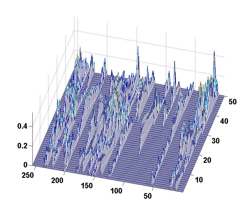
Experiment was repeated for 63  trials. The averaged results (from Time 0 to Time 60) are shown in the following pic (click the pic for large view):
Here we can see, both KF-CS  and LS-CS have large errors when the sparsity profile of the columns in X changes (indicated by the four large bumps). In contrast, M-SBL does not have this phenomenon and has much small errors in most duration. KF-Genie indicates the Kalman-Filter estimation when the support of each column in X is known.

The averaged elapse time is (in my notebook):
KF-CS is 168.5 seconds
LS-CS is 168.3 seconds
M-SBL is  19.7 second

I have to emphasize, if we segment the whole data into several shorter segments, and then perform M-SBL on each segment and concatenate the results from each segment, we can get better performance.

So, the conclusion is, the MMV model has great potential for the problem of time-varying sparsity patterns. This is somewhat like that people generally view each short segment of a nonstationary signal as a stationary signal. So, viewing a time-varying sparsity model as concatenation of several MMV models is probably a better way to solve the time-varying sparsity model.

Some of the results can be found in [7].

Reference:

[1] D.P. Wipf and B.D. Rao, An Empirical Bayesian Strategy for Solving the Simultaneous Sparse Approximation Problem, IEEE Transactions on Signal Processing, vol. 55, no. 7, July 2007

[2] Z.Zhang, B.D.Rao, Sparse Signal Recovery with Temporally Correlated Source Vectors Using Sparse Bayesian Learning, accepted by IEEE Journal of Selected Topics in Signal Processing, [arXiv:1102.3949]

[3] Namrata Vaswani, Kalman Filtered Compressed Sensing, IEEE Intl. Conf. Image Proc. (ICIP), 2008

[4] Namrata Vaswani, "LS-CS-residual (LS-CS): Compressive Sensing on the Least Squares Residual", IEEE Trans. Signal Processing, August 2010

[5] J.Ziniel, L.C.Potter, P.Schniter, Tracking and smoothing of time-varying sparse signals via approximate belief propagation, Asilomar 2010

[6] SF Cotter, BD Rao, Sparse solutions to linear inverse problems with multiple measurement vectors, IEEE Trans. on Signal Processing, 2005