Is MMV more suitable for dynamic environment (time-varying sparsity) than KF-CS and LS-CS? (3)

Previous experiments are based on the data generated by the file gendata_full.m in the LSCS_KFCS_code.zip. I noted that the data actually are not stable, since the data is generated by the command:
x(:,t) = x(:,t-1) + sqrt(Q1)*randn(m,1);
So, the energy will increase with time. It is interesting to see when the the system x(:,t) is stable (i.e. X(:,t)=P X(:,t) + V, with the eigenvalues of P are less than 1), what's the performance of the algorithms. The stable system is more often encountered in practical problems.

So, I carried out another experiment using stable data. Each coefficient time series was generated as:
x(i,t) = b * x(i,t) + sqrt(1-b^2) * randn(1), with b randomly drawn from [0.7,1).
So, each x(i,:) is a temporally correlated time series.

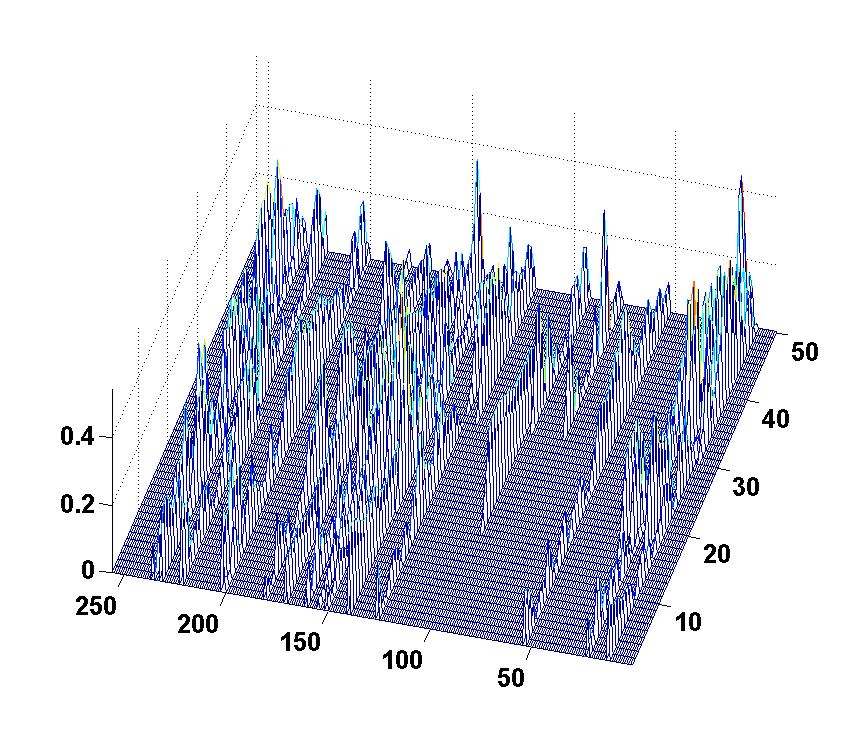
At initial stage, the number of nonzero coefficients were 15. The support of x(:,t) will change at t=15, 25,30. New 10 nonzero coefficient time series were added in the support at t=15 and 30, while 4 existing coefficient time series were removed at t=25.

A picture of the evolution of coefficient amplitude is given below (the label for the bottom axis is the index of coefficient; the label for the right axis is the snapshot index; the label for the left axis is the absolute amplitude):

The dictionary matrix was 60 by 256. The total number of snapshot was 50. Noise standard variance was 0.01 (about 20 dB). I compared KF-CS, M-SBL and my T-MSBL. KF-CS was performed on the whole data. T-MSBL and M-SBL was performed on 5 segments (I evenly divided the whole data into 5 short segments with 10 snapshots). Experiment was repeated for 25 trials. Here is the result:

We can see T-MSBL achieved the best performance. I am somewhat surprised by the behavior of KF-CS. Probably KF-CS's detection to disappearing coefficients is more sensitive to the pre-defined values. As for elapse time, KF-CS cost about 190 second, while T-MSBL and M-SBL cost about 3 seconds (note here the input argument MIN_GAMMA for the SBL algorithms was set to 1e-3, which was different to the values in previous experiments. Different values of  this input argument can result in significant change in speed).

The strange behavior of KF-CS in above experiment is probably due to the algorithm sensitive to the pre-defined threshold to remove disappearing coefficients. I used the threshold value given by the code, but didn't try other various values, because each running took much time. So, to remove the effect of this issue, I designed another experiment.

The experiment is an exactly MMV experiment, i.e. the support of each column in X didn't change (all satisfy the common sparsity assumption). Here is the result:

As in the above experiment, T-MSBL and MSBL were performed on 5 segments. And their final results were the concatenation of the recovered results from each segment. Again, we obtain the same conclusion.

So, I believe, for time-varying sparsity problems, dividing the whole data into several short segments and then using MMV algorithms on each segment is an effective method.

Referece:
Z. Zhang, B.D.Rao, Exploiting Correlation in Sparse Signal Recovery Problems: Multiple Measurement Vectors, Block Sparsity, and Time-Varying Sparsity, ICML 2011 Workshop on Structured Sparsity


-----
Another tulip is flowering in my patio: